Author: admin

After our introductory post  on Network Strategy, many people reached out to us asking about the distance formula that we used to calculate the distance between two points.

Distances between plants, DCs and customers are the key things that impact supply chain design and customer service levels. So, we have decided to cover this topic in a short post to arm you with all the ultra-useful tools you’d need to calculate the distance between two points. If you are just looking to calculate distances based on Latitude and Longitude of the two locations, you can directly skip to section 3.

If you are just looking for an excel file with Spherical distance formula with Lat-Long, download it here.

1. Cartesian Distance

2.Taxicab Distance/ Manhattan Distance

3.Spherical Distance (Law of cosines)

Cartesian Distance

Dusting-off our high school mathematics, there is a very direct formula to calculate distance between two points if you know their coordinates. Let us refresh our memories.

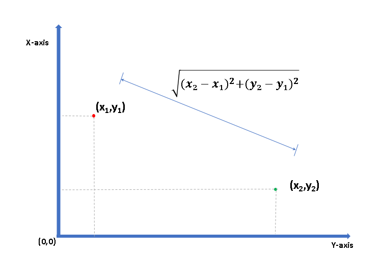
So if the two points are (1,5) and (6,2) respectively then the distance between them is 5 units.

Taxicab Distance/ Manhattan Distance

When we are dealing with planned urban areas, especially a grid of roads covering the city like Manhattan (hence the name Manhattan distance), we’ll have to travel along the grid to reach from one point to another.

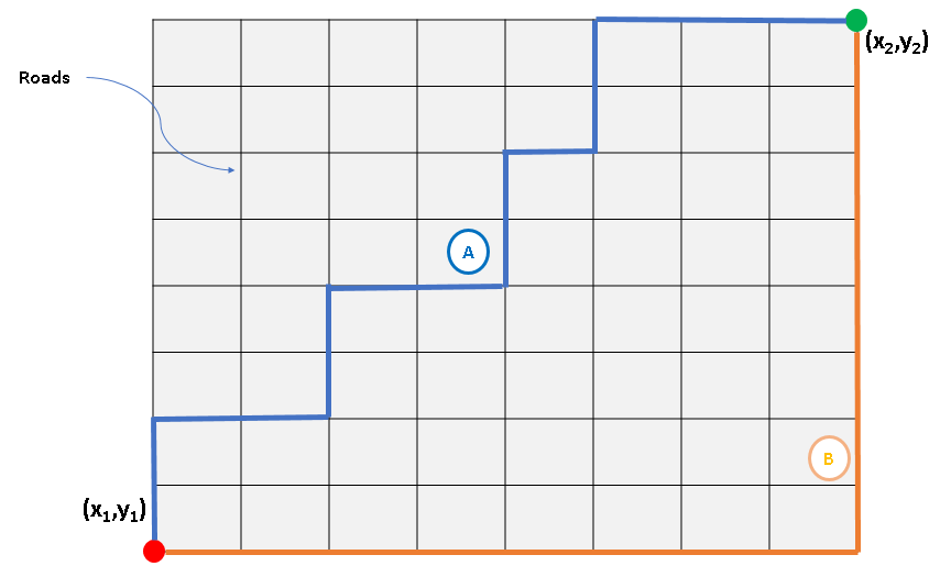
In such cases, the distance travelled is simply |x2-x1| + |y2-y1| and remains the same for all possible routes as long as we are moving towards the destination point. In the above example where the grid is 8 x 8 units, we’ll have to travel 16 units.

Taxicab distance or Manhattan distance is quite useful while calculating last mile delivery distances in planned urban areas.

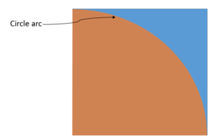
Spherical Distance (Or "As the Crow Flies" distance)

Question: What would you do if I asked to travel from point A to point B on the surface of the Earth in the shortest distance?

Answer: Dig a tunnel.

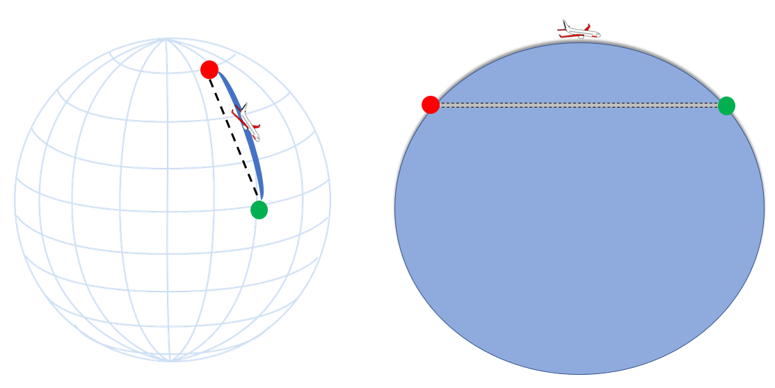
Earth is a sphere (unless you are one of these guys)  and even when you travel in a seemingly straight line, you are bound to follow earth’s curvature. And this is the reason we can not use the Cartesian distance for calculating the distance between the two points.

Then, how can you find distance between two geographic locations if you just know their latitudes and longitudes?

We use something called “Spherical Law of Cosines“ that gives distance between two points on a sphere.

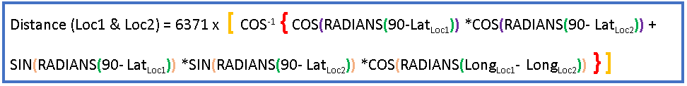
This formula may look complicated but it’s easy to implement. Download the Excel file to see this formula in action.

Assumptions

Circuitory Factor

The spherical distance formula gives distance “as the crow flies”. But roads are never a straight line – they zig-zag around natural obstructions and take detours to towns and cities on the way. To account for these curves of the road, we multiply our straight-line distance by a Circuitory factor. Typically, this factor is assumed to be 1.18

That is, the actual road distance is 18% more than the straight-line distance given by spherical formula.

This Circuitory Factor (also known as Detour Index) varies from geography to geography – coastlines and mountainous regions will have higher factor than plains.

For more details you can refer to other relevant articles here and here.

Earth isn’t a perfect sphere

Earth is an oblate, and that is the reason why neither the top of the Mount Everest is the farthest point from the centre of the Earth nor the bottom of Mariana Trench is the closest.

But this oblateness means  that our spherical formula isn't perfect especially over large distances.

Natural obstacles

While using the distance formula, be wary of any natural obstacles  that will have an impact on the route. This is especially true for mountainous regions, archipelagos, or any other regions where the movement between the two locations takes indirect routes.


Was this post useful? If you have any additional questions, feel free to drop a comment below.


Hola! Detectives. With the previous series of articles on inventory and service levels, it is time now to jump onto realms of some serious strategy stuff! Yes, I am talking about Supply Chain Network Strategy.


Believe it or not, majority of supply chain costs are locked at the time of fixing our network. You will have to continue paying rentals for our DCs, salaries need to be paid every month; and unchanging distance between DCs, plants and customers means that there is certain minimum transportation cost that we will have to incur regardless of our operational excellence. If your network is sub-optimal then you’re stuck with an inefficient supply chain with little to no wriggle room to improve on cost and service. Hence, a network strategy decision can make or break a supply chain.

Majority of supply chain costs are locked at the time of fixing our supply chain network

In the next few articles we will see how to design a supply chain network. We will cover the following topics:

I. Greenfield Analysis
II. Advanced Greenfield Analysis
III. Network Trade-offs
IV. Network Strategy v/s Organizational Strategy

Objectives of Network Strategy

Primary Objectives:

Secondary Objectives:


Greenfield Analysis

Let us begin from the simplest of the network strategy techniques – Greenfield Analysis. Greenfield analysis is relatively quick way to determine optimal locations for a given demand network. This is one analysis that you’d almost always do first especially when you don’t have any existing network to serve a given set of demand. In other words, a green field. Greenfield Analysis is also useful benchmark to compare the existing network to the ideal “optimized” one.

To understand this, let us start with a fairly simple example. Below is hypothetical scenario where our demand is coming from 10 different cities.

Question: Given these demand points where should be my production plants be located?
We want to know where should we open our plants so that these demand locations are optimally served? What should be the location(s) if I were to open only 1 plant? 2 plants? 3 plants? 4 plants?

Approach

The first step towards a “good” network is to have a clear and accurate blue print of your customer demand. It is important to understand who the real customers are and what is the real demand. Clean your data for any bull-whip signals or cyclicity.

Second step is to aggregate the demand at a logical level. While designing a country-spanning supply chain network, a reasonable demand aggregation could be city. Theoretically, we can of course model at the most granular level i.e. store or street, but it will require a significantly higher effort in data collection and modelling without much gain in the quality of the results.
Our demand data is already aggregated at the city level.

Third, on this cleaned and aggregated demand data we apply a technique called Centre of Gravity or CoG. As the name suggests, it basically means identifying a “middle point” of demand locations. It is intuitive too - we tend to live in places that are at the “centre” of offices, schools, shopping centres, hospitals etc. This is the same principal at work here.
For mathematically inclined – we want to select plant location(s) such that sum of distances from those location(s) to the demand points is minimal.
We did some Excel magic and voila! We have our COG locations –


Notice how the average distance decreases as we open more plants. If we open just one plant, the average distance to customer is 684 kms but if we open four, the average distance reduces to 218 kms. Assuming transportation costs to be proportional to the distance for this specific case, then adding three DCs to the network reduces the transportation costs by 68% !

Excel Modelling

So how did we arrive at those precise Centre of Gravity locations? The answer: Excel Modeling. We asked the excel solver to tell us COG locations so that the total distance between the COG location (plant) and demand is minimized. Download the Greenfield Solver here.

If you are new to Optimization and Excel Solver, I strongly recommend you to check out our previous article on this topic before reading further. Done? Good. Now let’s see how we modeled this problem in solver to give us COG locations.

1. Decision Variables

We have two key decision variables here
a. Location of plants: Latitude and longitude of the plants
b. Plant to demand mapping: Which plant should serve which DC

2. Objective function

Minimize the total weighted distance from factory to the demand point.
In other words: Minimize Σ (Demand at a region x Distance from COG)

3. Constraints

a. Number of Plants should be equal to as desired by the user
b. Demand points should be served by exactly one plant
c. Latitude variable can vary between -90 deg. and +90 deg.
d. Longitude variable can vary between -180 deg. and +180 deg.

Feel free to play around with the model. However, be warned that due to non-linear nature of the problem, solver takes a long time to solve particularly for 4-COG model. For reference, it took 30 mins to solve for 4-COG model at moderate tolerance settings. (i.e. we asked solver to give us a “good” solution rather than a perfect one which would take even longer to solve.) 

It will be quite difficult to solve a 5 or more COG model without moving to more advanced solver engines or tools. There are many advanced tools in the market that are highly recommended for thorough network strategy projects. We will look at some of these tools in the later articles in the same series.

Conclusion

COG is used in various ways – apart from getting potential locations from scratch, you can also use it to compare the efficiency of your existing network. For e.g., let’s say that we had an existing network of 4 DCs for the demand locations that we just saw now, but at different locations than what greenfield recommended. And if we know that the average distance in that network is 400 kms then we can state that we traveling an extra 180 kms to service the same demand! Against 220 kms that an ideal network delivers. And this inefficiency translates into additional costs and lower service levels.

So, now we have got four answers for the COG problem. We know where we would put our plants if we were to open 1,2,3 or 4 plants. But then the next big question arises - What is the correct number of plants? Should I open four small plants across the country or just a big one at the centre? Or something in between?

Don’t worry – your SCD journey to become a Ninja level Network Strategy Expert has just begun. Keep tuned in for the next article in series and subscribe to our blog to get notified.


Was this article useful? Let us know through your comments.


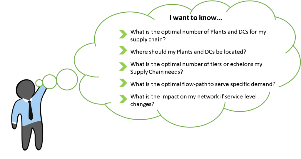
Have I landed on a wrong blog by mistake? Why the heck we are talking about finance on a supply chain blog?

If you are thinking that, consider this harsh fact – supply chain is a cost center. Supply chain doesn’t sell anything. Heck, supply chain folks are often found in the alleyways of 5-star hotels screaming at the transporter in the choicest words, while inside sales guys are receiving performance awards for delivering their sales targets.

But jokes apart, any supply chain initiative must be backed by financials unless you want it to be shot-down in the crib. No one is going to give you money for extravagant warehouse robots  unless it makes for a solid business sense.

And to do that one must be aware of basic financial modeling and concepts. Let us illustrate it through an example.

Problem

Your organization is contemplating buying a new fancy line of warehouse automation systems. This includes an automated picking and a conveyer system. Though all your simulations show an improved performance of your warehouses, the system is expensive and your CEO has asked you to prepare a business case.

Sensing your cost consciousness, the vendor Buy-It-Already-Sucker (BIAS) Pvt. Ltd. has offered you three business options:

While the first two options are straight forward, the 3rd option is “Rent & Buy” which means that you’d be paying $ 250,000 per annum and by the end of six years, you’ll own the asset. Additionally, there is a 4th hidden option too (and default option for procrastinators): Maintain Status Quo, i.e. don’t do anything.

Now with these 4 options in your hand, your next objective is to:

One – Prepare a business case with financials that will convince all the stakeholders

Two – Select the most profitable option

On the face of it, renting cost seems high but to buy the asset, we’ve to pay $ 1 million right now, which might not be as easy. However, option #3 looks quite attractive where we’ve to pay same as rental but only for 6 years and then the asset will be ours. But NEVER FALL IN THIS TRAP of making an important decision on intuition without doing the numbers.

So how can you compare these options? We’ll use a technique called Net Present Value (NPV) or Net Present Worth (NPW) calculation. If you are already familiar with this concept, you can skip the next section.

NPV Calculation Basics

Would you rather have $10 dollar today or $10 dollar tomorrow?

Of course, you’d rather have it today. “A dollar today is worth more than the same dollar tomorrow.” And this is the basic fact around which the whole financial world revolves. If you expect people to accept money later you’ll have to pay a little bit extra, which is called interest.

Let’s say that you agree to pay someone $11 tomorrow in exchange for their $ 10 today. This extra $1 is the interest and you just paid 10% ($1/$10) as the rate of interest.

Similarly, $ 12 tomorrow is worth...$ 12/(1+rate of interest) = $ 10.9 today. This $10.9 is Net Present Value of $ 12 of tomorrow.

Comparing the above two examples, using the rate of interest as 10%, now let me ask you a slightly modified question - Would you rather have $ 10 today or $ 12 tomorrow?

Now, you’d choose $ 12 tomorrow, since we know that Net Present Value of $ 12 is $ 10.9.

Using this logic we can calculate the NPV of all the future cash flows to compare the possible options.

NPV Model

To build a NPV model, we’ll go through five simple steps:


Step 1: List all future inflows and outflows

In a strict sense, productivity savings and damage reduction are not inflows. However, relative to our base case of "do-nothing" (option 4), which we are assuming to have a zero NPV, these are cash inflows for the organization.

Step 2: Estimated value against all inflows and outflows

Pro-Tip: It’s always useful to keep input values dynamic in the model. This is because things change, and you don’t want to recreate the whole model when one of input changes. E.g. you may realize that life is asset is not 10 years but 2 years.

We highly recommend 13 Tips and Tricks for Excel modeling for more such Pro-Tips.

Step 3: Identify other external factors (e.g. inflation)

There can be scores of other external factors that impact your future financials. Prime example is inflation. For our current example, we estimate that inflation is going to remain at 5% and it will impact maintenance, operational costs, and reduction in value of damages (not because inflation impacts the damages directly but because we assume value of damage products to increase @inflation)

Step 4: Estimate Cost of Capital (interest value)

Organizations receive money from several sources, shareholders, banks etc. They expect a decent rate of return to compensate for the risk they are undertaking. We assume this to be 18%  for our example.

Step 5:  Bring all the cash flows to today’s value (NPV) and compare different options

As you can see below, we’ve shown cash flows for the first 6 years for the buy option. the light red  shaded cells show outflows and light green are inflows. The gray cells show the net.

Download the complete excel model here.

Few other things that you can observe above:

- Maintenance is free for first 5 years as given in the BIAL quote. It’s, however, applicable from sixth year onwards

- Maintenance and operational cost increase @rate of inflation

 RESULTS AND CONCLUSION

If you haven’t, download the entire model here.


Are you surprised with the results? I was.

After doing a detailed analysis, we find out that Option 1 “Buy” has a positive NPV of about $ 42k. Even better is Option 2 “Rent” that has a NPV of $ 112k. Hence, we should go ahead for option 2 and RENT the conveyer system.

Interestingly, our initial hunch for Option 3 “Rent & Buy” was gravely wrong which is not only worse than Buying or Renting, but has a negative NPV of $ 56 k. It demonstrates how these decisions shouldn’t be done on intuition but on the basis of logic.

We hope that this article enhanced your understanding of NPV and it’s role in decision making. Feel free to play with the excel workbook. Tweak the inputs and see how that changes the NPV of different options. Found an interesting combination of inputs that gives surprising results? Share with everyone in comments.


Our previous article on Simulation, unexpectedly, became the most popular post on this blog. Thanks for your love, fellow SCDs.

We also received several e-mails on the topic and they can be broadly classified into two groups.

One group’s feedback went something like –

“I loved your post on simulation. However, I wonder if simulation can only be used for “what-if” analysis or there are other applications too. Nevertheless - a big fan of your work. Hugs and kisses.” (partially exaggerated)

While the other set of responses were less flattering –

“What a load of BS! In what world the customer demand is non-random with a forecast accuracy is 100%. This SCD guy should shut down his website and get a taste of this cruel world. Eat dirt, you phony.” (partially censored)

And to both kinds of people, my simple two-word answer is – MONTE CARLO SIMULATION.

What is Monte Carlo Simulation?

Monte Carlo Simulation is a simple yet brilliant technique where results from several thousand iterations are aggregated to arrive at the solution to an otherwise difficult problem. A common theme of Monte Carlo Simulation is that the input uses random variables. It has been used from simple probability problems to simulations for Manhattan Project.

We can fill pages of theory on Monte Carlo but, as you know by now, here at SCD, we love learning by examples. Today we’ll do three Monte Carlo Simulations and if you understand the logic carefully, you’re guaranteed to achieve the reverence in your professional circles. But don’t get intimidated, we’ll start with super basic ones.

Example 1:  Finding probability of getting “7” in random roll of two dice

Example 2: Calculating the value of π

Example 3: Finding the required Safety stock for a target service level

Example 1: Probability of a sum from two-dice roll

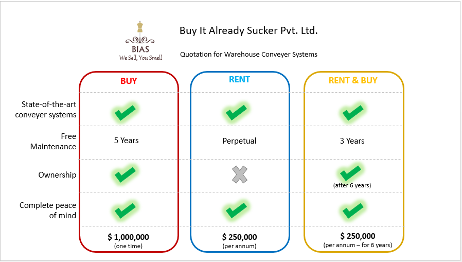
Let us start with a very simple example– we have two sets of standard six-sided die with us. We would like to know what are the chances of getting a total of “7” when we roll them. You can get seven by several possible combinations, say, by getting “5” on one die and “2” on other, “6” on one die and “1” on other. In fact, there are more ways to get “7” than, say, getting “2” which can only be achieved in one way - by rolling “1” on both the dice.  So intuitively we know that chances of “7” is higher than “2”, we don’t want to do any mathematics to arrive at the probability. How then, in the name of Fermat, can we calculate it?

Ummmmm... we can roll the two dice a large number, say, fifty-thousand, times and count how many times we get “7”.  Well, that’s what is Monte Carlo simulation. 

Using MS Excel and its nifty RAND() function, we imitated throwing of two dice fifty thousand times and plotted all the values in a nice Frequency Table.

As you can see “7” occurred a total of 8353 times out of 50,000 tosses. That is 16.71%.

Now, your mathematician friend (what, you don’t have one? Get one. Those are good to keep around in case you are planning to visit some casinos) will tell you that probability of getting “7” from two-dice throw is 1/6, which is 16.67%.

Our simulation gave a very close answer without knowing an iota of probability theory. This is the real power of Monte Carlo simulations. You can download the file and see it for yourself by re-running the simulation by pressing F9. You can also achieve even more accurate answer by increasing the number of rolls.

Example 2: Find π (by throwing darts)

You read that correct. Monte Carlo simulation can be used to calculate nature’s little irrationality by one of the most simple yet brilliant simulation this SCD has ever seen.

Imagine you have a square dartboard. Now inscribe a quarter circle on the dart board such that, the radius of the circle is same as the side of the square. Let me draw it for you.

Now, what is the ratio of two orange shaded area (circle) and the square? Easy-Peasy. 

With us till now? Good.

Now, let’s have a little friendly game of darts using that square board. Don’t think too much...just take out a bagful of darts and start throwing. Bam! That’s what I am talking about.

But don’t stop just now...you have to throw 10,000 such darts at the board. Being a lousy thrower you are, darts have landed across the board randomly either inside or outside the circle.

Now you know that larger the area, larger are the chances of dart landing inside. In fact, if you throw large enough number of darts, the fraction of total darts landing inside the circle is equal to their corresponding areas. And we know already that the ratio of areas is equal to π/4

Using the above formula and little magic of excel, we can calculate the value of pi.

See the results of simulation below.

Download the file and feel free to play with it. As you can see, the pi values are in the ball-park. However, you can improve it’s accuracy by increasing the number of “darts” in your simulation.

Example 3: Safety Stock Optimization

We’ve saved best for last. Have you ever been in a situation when you solve a complex business problem (any business problem) by digging into tons of research papers, highly referred books, and top cited material, only to be scoffed at your results by the decision makers just because they don’t understand it? If you haven’t, you WILL be.

This SCD was delivering an Inventory Optimization project for a client when he applied some advanced safety stock calculation formulae to generate inventory recommendations. An unconvinced stakeholder looked at the long list of Store-wise, SKU-wise, inventory recommendations and said –

“What is this mumbo-jumbo with µ’s and sigmas? And are you suggesting that we keep twice the inventory than our average forecast? Are you crazy or what? We will just keep 7 days of inventory as we always have and that’s it. Period.”

How can you convince this guy?

Of course, Monte Carlo Simulation. This SCD created a simulation to show how the customer demand is distributed and how he needed that amount of safety stock to meet the customer service levels – WITHOUT USING A FORMULA. We’ll take you through the step-by-step process on how this is done.

Download the file to follow the next steps.

1. Define inputs

Assuming that demand follows a normal distribution, we need the following values as input – Average demand, Standard Deviation of Demand and Target Customer Service Level.

2.Simulate the random demand

We want to have a randomly distributed demand following the normal curve. Excel functions of Norm.Inv() and Rand(), can help us generate these random demand points. You can refer to the attached excel sheet for the exact formula.

This demand pattern is something we want to show to our beloved stakeholder because they can easily relate to it without going into the formulas. We have generated 10,000 such random demand points and also plotted them on a Frequency Chart.

As you can see in the graph above, the most frequently occurring demand is around the average i.e. 200 units. Secondly, as we move further away from the average on either side, the frequency of demand point reduces – this is, in fact, a typical normal curve.

3.Calculate ‘Find’ Safety Stock

The beauty of Monte Carlo Simulation is that we don’t have to calculate anything. We have a long list of possible demands. We also know that we want to fulfill 95% (customer service level) of all those possible demands.

We can sort those 10,000 demand values in ascending order and select the 95th percentile from the top. Thankfully we have a ready-made formula in excel called PERCENTILE.EXC to find that value. And Voila! This is our total inventory requirement.

So, 95th percentile value corresponds to 240 units of stock. Out of this average demand is 200 units, and remaining 40 units is safety stock. Corresponding fill rate is 99.72%.

The logical flow in this spreadsheet is far easier to explain to anyone. Show a list of randomly generated demands. Ask how many of those demands organization wishes to fulfill and POP! That’s the stock you need.

Download the file if you haven’t already. Go ahead – all the values are dynamic so have fun playing with it.

BONUS CONTENT!

We can’t give enough. Can we?

We just found out stock levels for a given customer service level. What if we were to flip this problem? What if we were to find the customer service level that can be achieved for a given inventory level? Something that can get us following output.

Try making a Monte Carlo model yourself OR download the simulation and analyze the solution. Enjoy!

Did you like this post? What are the other problems where you think you can apply Monte Carlo technique? Let us know through your comments.

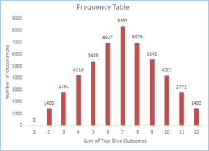
Whenever you pick-up that joystick for shooting aliens, running through cross-dimensional portals or hopping Italian plumbers through the obstacles to save make-believe princesses, you are running a simulation. Examples of simulations go well beyond video games – armies across the world use simulation to train their soldiers; trainee pilots are first put on flying simulators and some people even believe that our entire Universe is a simulation.

But what is a simulation?

If you open a book you will see a definition of simulation something like:

"Simulation is an imitation of a closed system over time under pre-defined rules."

...at which point you’ll promptly close that book and go back to shooting aliens.

At SCD we like to define simulation as –

" Modeling some crazy and not-so-crazy fantasies of management executives and running what-ifs before actually implementing them and risk burning the whole company to the ground."

Simulation has a wide range of applications and we can go on and on singing peans about it, but why not take up an example problem and solve it together so that you see it for yourself? Sounds good? Here we go...

PROBLEM

After you helped Han Solo maximize his profit on planet Excel XIII, you’ve become a blue-eyed boy of Supply Chain VP. But great performance comes with great expectations. And being the top-notch SCD that you now are, you are getting involved in high-stakes problems.

Here is the situation – your company has two stores and in general things are going well for them. They sell stuff to customers and whenever they want, they can place an order to the factory. However, the only constraint is that they have to place an order of minimum 500 units (MOQ). Now, your Supply Chain VP has this latest brainwave where he wants to increase this minimum order size to save on transportation cost.

He has a hunch that increasing this MOQ from 500 to 750 will save him a lot but he isn’t sure because doing this will also increase the inventory throughout the system.

So he wants you, dear SCD, to run a simulation to understand the overall impact of the system if he chooses to go ahead with the decision.

As you ponder upon this new problem that has been thrown at you, you are caught somewhat unprepared. You know that you can’t use the old tricks (like optimization) but sticking with the basics and some application of mind, you’re sure you can come up with a simulation model.

But before you begin, you want to know the exact details of the operations at the stores so that you don’t miss out on any of the variables or relevant data. Well, a perfect opportunity to use your acquaintance with the store manager.

You’re glad that you had this chat; you are now wiser about the store operations and have an idea or two about modeling this simulation.

You take out pen and paper and try to come up with a step-by-step plan.

Step 1: Identify the Key Indicators that you want to monitor during simulation

Key Indicators are basically output variables that you want to see the impact on. For e.g. what would be my transportation cost under the new policy?

Don’t worry about how you’ll calculate them. Think from your boss’s perspective on what he’d love to see to make it easy for him to make decisions. These Key Indicators also called “Targets” or “Actors” by certain advanced software, can pertain to supply chain, finance or any other function. They can even go beyond your organization to capture overall system impact.

You make the following list:

Transportation Cost

Inventory Cost

Total Orders placed

Step 2: Identify the Base

There are multiple inputs that can go into a simulation model. But there is often one input that forms the “base” for simulation. You can consider this to be the “independent variable” or the X-Axis that will “pull your model”. This can be the Demand, Forecast or simply Time. For e.g. when your local weather department gives a hurricane warning, they are essentially simulating the path of the hurricane with respect to Time.

Img Source

You think long and hard...what should be the “base” for your simulation?

You rewind the whole conversation with the store manager...and as if on cue, a new mail pops up on your screen. The store manager had sent you day-wise, store-wise sales data.

That’s it! Your simulation model must simulate the day-by-day demand at the stores and see if an order needs to be placed! That becomes the base for your model1.

Download the complete file Here.

Step 3: Identify other inputs

What things impact your model? What are the other “numbers” that you need that are needed for you to make an ordering decision?

Lead Time (in days)

Inventory Carrying Cost in percentage

Item Cost per unit (to calculate inventory costs)

Transportation Rates (per trip)

Opening Stock

Step 4: Define simulation rules

Aha! This is the most interesting and most challenging part of simulation modeling - rules are essentially the engine that drives your simulation. When you are playing a video game, it also follows some rules –

Pressing button A will fire the gun, if there is an alien in the path of the bullet, he’ll take damage OR

When Mario jumps and catches a mushroom, he’ll double in size OR

When the hurricane encounters warmer air, it becomes more powerful

You jot down the following rules for your simulation

1.An order must be placed when existing inventory is not sufficient to cater to next n days of cumulative demand, where n is lead time

2.The order quantity should be at least MOQ units (500 or 750)

3.Demand depletes the existing stock

4.Every trip costs X dollars

THE MODEL

With some trial and error, but following the modeling basics, you come up with a beautiful simulation model.

Download the model Here. You can also download vba free, but completely functional, model Here.

Also, summary of results for MOQ 750 vs 500 is also given below.


You watch your boss as his eyes widen and face exudes almost an orgasmic look as he sees that MOQ simulation. Not only he sees 30% reduction in overall costs, he can also tweak ANY inputs and see the results live! Well Done, SCD!

CONCLUSION

“A flutter of butterfly’s wings can ultimately cause a typhoon halfway around the world.” – Chaos Theory

This phenomenon is called butterfly effect. But what does it has to do with simulation? Everything. Butterfly effect applies to the organizations too. At times, people are so involved or invested in certain decisions that their visions become limited and they fail to notice a far-reaching consequence for their organization or even other organizations. This is where simulation comes in handy. It often throws surprising results and it can help quantify what seem like unsolvable problems.

For businesses and especially for supply chain professionals, simulation is as powerful tool as optimization, if not more. Especially before taking high-level decisions, running a simulation can help discover any side-effects and potential implications.

In fact, this SCD has used simulations to calculate the value of pi (more on this in a later post), assess warehouse requirements, quantify the impact of changing vehicle mix and many, many others.

Have you used simulations for your business problems? Or you are stuck with a business problem that seems too difficult to solve normally – simulation might be the answer. Do let us know through your comments below.


Footnotes:

1 There are a couple of inherent assumptions here. One, we have assumed that sales = demand. This assumption is invalid if we had stock-outs in our warehouses. In that case, we use a technique called “data imputing” to put approximate values for the missing data.
Two, since we are using the historical data, we have the advantage of hindsight, that wasn’t available to the poor planners while placing the order. Hence, it’d be unfair for us to directly compare the actual results (with old MOQ) vs what-if results (with new MOQ) in such situation.
There are ways in which this simulation can be made fair – one, we can use the forecast that was used while making earlier decisions. Two, we can run the what-if with old MOQ itself and Three, make demand as a random variable following a given pattern.
In our current simulation, we are using the second technique where we are running the simulation with old MOQ itself.

Life is replete with trade-offs. Whenever we take any decision we have to think about all positives and negatives.

Shall I live closer to the city to save on commute OR live on the countryside to save on rent?

Shall I buy a smaller quantity to save on my inventory costs OR buy in bulk to save on ordering costs?

Shall I marry the girl who is more beautiful and rich OR the one who is more intelligent, empathetic and caring?

While the last trade-off can’t be evaluated by Excel modeling...

Alt Text


...never mind.

Whatever is the problem, we have to evaluate trade-offs involved to arrive at the most reasonable answer. An optimized answer.

There is tons of theory that goes behind Linear Programming and optimization, but this SCD thinks that best way to understand the concept is through a story. And what better story than one that is worth $ 42 billion.

PROBLEM

Han Solo and Chewbacca, smugglers in a galaxy far far away, while trying to dodge the troublesome Imperial law enforcement, have landed their famous spaceship the Millennium Falcon on an unknown planet called Excel –XIII. While searching for a good place to go underground, they encounter a trader who is selling some interesting stuff at a good bargain.


However, there are some big constraints because of which he can’t buy everything on offer.
Han Solo, never to miss out on a good money making proposition, realizes that he can make a profit on all the items listed above with the trader.

1.His spaceship doesn’t have space for everything (he only has 20,000 cubic cm)

2.He doesn’t have enough money to buy everything (he only has 10,000 credits)

Being a shrewd smuggler and a businessman that he is, his objective is to optimize this deal and maximize his profit. He quickly adds more information to the table:


As we can see above he has added three more columns

Space requirement – that tells us how much space is needed for each unit of the item

Potential profit – that tells us how much profit Han Solo stands to earn by selling that item elsewhere and,

Potential demand – that tells us how much quantity of that item that Han should be able to sell

He realizes that manually figuring out what items he should buy and in what quantity would be a mammoth task that’d take him a long time. Fortunately, he is on the planet of Excel-XIII where he has the right tools at his disposal. With Chewbacca's help, he decides to build an Excel based optimization model.

Download the file with the model.

Han knows three steps for modeling any optimization problem. So, he jots down the following:

Step 1: Identify the decision variables

Decision variables are simply the things we want to solve for. For e.g. Han wants to know which items he should buy in what quantity.

He the adds another column to the table, called “Buy Quantity”. He doesn’t know the values yet so those values remain blank. In fact, he wants the magic of optimization to fill in these cells for him.

Step 2: Write the objective function

Objective is nothing but the ultimate goal we are trying to achieve. Maximising profit, minimizing the cost, maximizing the score in our girl selection problem are some examples of objectives.

For Han, it is to maximize his profit from the proposed trade.

When objective is represented mathematically it becomes an objective function. E.g. Sales x margin, production x cost etc. are the examples of objective function

Han puts a formula in the cell that calculates his profit. This is the sum of profit from the all the items that he is planning to buy. Though there is a formula there, the value in the cell is zero since there are no values in the “Buy Quantity” column that it uses as one of the input.

Step 3: Identify the constraints

Han would’ve bought everything had there weren’t any constraints. But sadly he does:

Constraint 1: His spaceship doesn’t have space for everything. He has only 20,000 cu cm.

Constraint 2: He doesn’t have enough money to buy everything. He has only 10,000 credits.

Apart from these explicit constraints, there are some hidden constraints that you simply know from common sense but we have to explicitly tell the computer. Remember that famous adage from the 1990’s that said: “Computer is loyal but foolish servant”.

Constraint 3: Han can’t buy more than what is available with the trader.

Constraint 4: Han can’t (or rather shouldn’t) buy more than what he can sell.

Constraint 5: Buying quantities can’t be negative.

Constraint 6: Buying quantities have to be an integer.

Solver Set-up

Alright, so you have successfully set-up the whole model. You’d be happy to hear that that was the toughest part of optimization. Now, you have to just run - something very appropriately called - “Solver”, that will evaluate these trade-offs, work under the constraints and optimize the objective by changing the decision variables.

But first, where is this magic called “Solver” you might ask. Don’t worry – “Solver” add-in comes free with all excel and you can find it under the Data tab.

If you don’t see it just head down to File --> Options --> Add-Ins --> Manage --> Select “Excel Add-ins” from the drop down --> Go --> Check the box “Solver Add-In”

When you click on “Solver”, you’ll get the following pop-up box.

Now we have to tell the solver about our decision variables, objective function, and the constraints. We strongly recommend that you try to model alongside using the model you just downloaded.

Step 1: Set Objective

Step 2. Select decision variables

Step 3. Add Constraints

Step 4. RUN!

This is the most fun part where you click solve and see the Solver run through several decision variables. Download the file with optimized values here

Voila! Han has the optimized quantity he must buy for each of the items. His profit will be 14,280 which is a great return on his original investment of 10,000.

We can also see that he is running out of money rather than space. Hence, money constraint (Constraint#2) is called a limiting constraint while space is a non-limiting constraint.

Take your time with the model and experiment with it. Change the constraints; tweak the objective function or try to relax a few constraints and observe how it changes the results. Try to think the problems for which this can apply to your organization. Analyze the solution reports.

CONCLUSION

Supply Chain Management is all about trade-offs – be it high stakes network optimization problems, tricky buy vs source decisions or cumbersome manufacturing line allocations – LP modeling and solver is one of the most powerful tools a supply chain professional can have at his disposal. In fact, the moment you’ve practiced a few problems, you’ll find its applications literally everywhere. Therefore, it can’t be over-emphasized that an expertise in LP modeling makes the difference between a Supply Chain Zombie and an awesome SCD.


Welcome back SCD!
I believe you are still basking in glory after creating an  awesome warehouse requirement model much to the pleasure of your boss. But you know what, we are just getting started– and you’ll soon find yourself encountering much more complicated problems. But don’t you worry; the five-step process that you learned in previous article, remains valid for all complexities and scales.

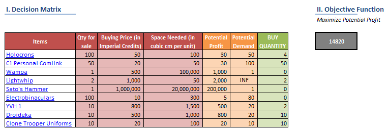
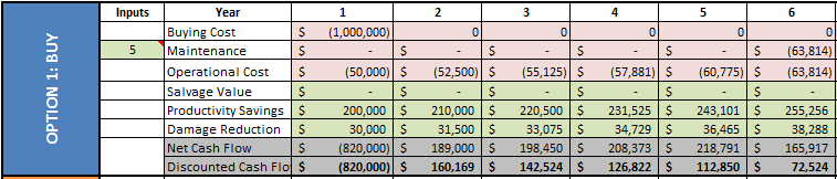
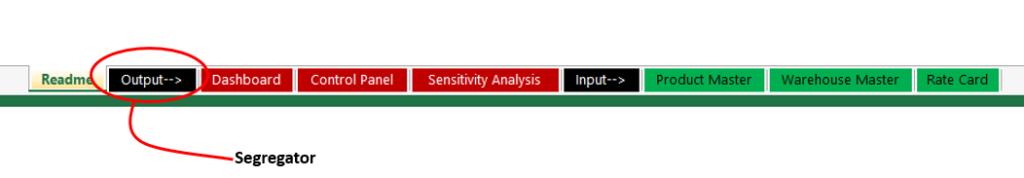
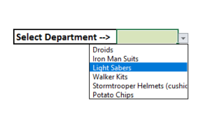
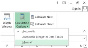
In this post, we’ll be looking at some tips and tricks that will improve your model structure and polish rough edges in your model. Individually, these seem like minor tidbits but sooner you inculcate these “hacks” as part of your day-to-day work, sooner you’ll realize that your thought process has become much more structured and your output significantly better than your colleagues. With some practice, before you know it, you will be that rare person in your organization who can translate seemingly insurmountable data into brilliant insights.
1. Color code your tabs and fields
Color coding your tabs and fields provide an instant visual cue to anyone looking at your model. In our previous model, we had input tabs as well as input fields colored in green.

2. Use “Name Boxes” to name your variables
This is one of the most useful functionality that most people either don’t know about or simply don’t pay enough attention to. You can name your important variables with meaningful names like “Pi”, “TruckingCost”, “TargetGrowth” etc. and then you can simply use this name in your formulas rather than referencing the cell where it is stored.

This name can be used anywhere in the workbook making your formulas easier to understand and also reduces chances of an error or wrong referencing.

3. Segregate input, output, and working sheets
If needed, you can add segregation sheets between various tabs of your model.

That way you can find all the related tabs and one place and keeps things structured.

4. Never hard code important inputs
If there is one thing that prevents your model being used by wider audience is lack of flexibility to change important inputs. There will always, I repeat always, be some inputs that are prone to changes. For e.g. in our WH model, though the departments gave you one single number for growth, no one would be sure if the growth will be 5% or 10% or 20%.
Don’t hard code such numbers and put such inputs as variables, preferably somewhere near the result tab where you can easily change them and see the results.
Another example could be currency exchange rates - you may be tempted to directly convert the currencies inside a formula itself, but taking time and effort to make it a variable pays off in such cases, since you don’t know when you’d need to change these variables or when your model will be used.

When you variabalize important inputs, you can be rest assured that your model can be used by the organization for years to come.

5. Use data validation functionality
This is another functionality that is often overlooked by most users. Data validation is a very useful while getting user inputs. You can have a drop-down list where the user can choose a relevant value. You can also have message pop-ups if the user enters invalid values.

6. Provide a readme tab
If you expect your model to be reused by a large number of people across the organization (In fact, you should aim for it), add a readme sheet in the beginning, explaining what model is doing and how a user can go about using it. You can also use this space to document all your assumptions.
Lastly, do provide your contact information so that they can approach you in case they identify bugs or have any suggestions or simply want to say thanks. It’s also a great way to get your name on your work.

7. Clear the clutter
You can make your sheets, especially the dashboards and output files look cleaner by
a. Hiding gridlines, headers, formulas and ribbon
b. Hide additional rows/columns
c. Hide working sheets that are not relevant to the audience
It also gives you more visual space and reduces the possibility to users unnecessarily poking in your working sheets.

8. Present your data in a form that is most useful to the audience
Understand your audience first and present your output accordingly. In fact, everything in your output dashboard should reflect the needs of that audience. For e.g. let’s assume you are presenting vehicle utilization data. If your audience is 3PLs representatives, then you want to show it to them by vehicle type and transporter. However, if the audience is the CEO, you want to show it by region along with competitor’s numbers.
Ask yourself a few questions beforehand:
a. What is the most important information for that stakeholder?
b. What are his/her KPIs?
c. Where do you want his decisions to be focused?
d. Who are the other people in the room? What questions can they raise in the room?
Additionally, if you aren’t confident of certain input parameters, you should keep those parameters along-side the output so that it can be changed “live”.

9. Stress test your sheets
Whenever you are giving a live demo, there will be at least one over-enthusiastic participant who’d want to solve global poverty through your excel sheet. Especially, if you’ve provided many user controlled inputs, some people will invariably be tempted to move the dials to 11.
Mr. SCD, what would happen we move that growth rate to be 100% and cost reduction targets to be aggressive 40% and ...
When you give them a hammer, everything will look like a nail. Your job is to either
a. Not give them more powerful hammer than needed. (Restrict user inputs to a certain range. For e.g. in the warehouse space calculation sheet, the slider can only be used to select years between 2020 and 2025) OR
b. Have your nails ultra solid. (You test your outputs to see that nothing breaks for extreme input values)
There is a highly discouraged third option too. Don’t even consider it! 1

10. Be ultra careful with external work-book references
Quite often, the model perfectly works on your system but when you send the file out, people begin to complain about ugly error message smeared all your hard work. This happens when writing your formulas, you referenced another file on the system. These formulas are unable to calculate as it can’t find that data at the other local machines and throw up an error.
For such cases, consider making those datasets as part of your model.
Even otherwise, especially for super-high level presentations, it’s a good idea to test it beforehand from other machines.

11. Validate formula after every step
I’ve noticed some people treating excel modeling similar to writing a story – they want to finish it first and then do the “spell check “later. BIG mistake. Large models have several logical steps working in tandem and in the case of errors, tracing back the mistakes across sheets could be a nightmare. Even worse, you may not see anything weird in your final output and mistakes may remain under the radar untill its too late.
So, cross check your formula results, manually tally couple of your vlookups, glance at the quick sums and counts at the bottom right of the sheet before going to the next step.
Additionally, formula auditing (esp formula evaluation) functionalities of excel can be quite handy to check your formula logic.

One extra minute spent in validation can save you hours of debugging later.
12. Disable auto-calculation
Every time you change even the slightest thing on your excel sheet, everything in your workbook re-calculates. If your workbook is large and formula heavy, each such change makes your workbook refresh for several seconds. When your workbook reaches such size, disable auto-calculation of the workbook to make it faster. Don’t forget to refresh it manually (F9) when you want to see updated results.

13. Data Management
This last tip is perhaps THE most important one. You can build a Ferrari of an excel model but it’d be utterly useless if you don’t have a quality raw data to fuel it. Hence, one of the first things that one should check before embarking on modeling, is data availability and data quality.

13a. Check for data availability
Having data vs no data can make the difference between
a. Looking for a black needle. In a black haystack. On a moonless night. Blindfolded. Hand tied.
vs
b. Looking for a black needle. In a white room. With a giant magnet.
Hyperbole aside, after you list down all the inputs you need for modeling, talk to stakeholders and see if the data is even captured. If possible, get a sample data-set beforehand. If the data is not available, you have two options ahead of you - make some reasonable assumptions or select suitable proxies that can be used as an input. For e.g. in our previous warehousing model (view post, model), let us assume that Droids department fails to give their future forecast. Without growth numbers, the model simply can’t work. Hence, we have to search for an appropriate proxy.


One such proxy can be organizational growth. We can take the average of other departments and use that to plug into Droids growth numbers.

But this is obviously a workaround and should be used with caution. If the confidence of the stakeholders is low for using certain numbers, consider adding sensitivity analysis to it.

13.b Data completeness and Data accuracy
What is worse than having no data? Think, think.
No?
Having incomplete or inaccurate data.
This might be counter-intuitive but it becomes clear when you think about it. If you don’t have the data you know that you don’t have the data. You can find some workaround, search for other data sources or try to plug the gap by hook or crook.
BUT if you have incomplete or incorrect data, there is a good chance that you won’t even know that there is something amiss. And you’ll continue to merrily use the data to churn out wrong outputs.
This SCD found this out the hard way. In one of the consulting projects, we found that output didn’t make much sense to high-level client stakeholders. They thought that there was a logical problem with our model while we couldn’t find any error with it. After couple of days were lost in stand-off, the issue turned out to be with the raw data. The data extraction query that one of the analysts had run, had stopped in between having extracted only about 80% of the transactions. No one realized the incompleteness of the data till it was very late.
Fortunately, there is a very straightforward way to mitigate against such disasters– Data Playback.
Whenever you get any kind of large-scale data, before immersing yourself with modeling it, summarize it in a way that can be easily recognizable by the relevant stakeholders. When you play their data back to them, they will instantly tell you if the data is incomplete or inaccurate. And your conversation during the play-back will go something like this:

SCD: So as you can see in the table above, we have summarized the sales data provided by your IT team. Does it look alright to you?
Stakeholder1: Well, everything else looks more or less fine but I don’t think we sold $xxx worth of lightsabers in the south.
Stakeholder2: I agree, I remember not meeting my target in that month. But wait, have you considered the product returns in your data. We had some quality issues in our south factory and had to do a mass recall of multiple batches of lightsabers.
SCD: Aha! I think that must be the reason behind mismatch of numbers. If we can get the returns data, I’ll use that to net-off the sales. In fact, it’d make much more sense to use the net sales instead of gross ones.
Stakeholder 1: Makes sense. I’ll get one of my guys to send that data to you.
SCD: Cool! And we’ll use the net figures in the model. Glad that we caught this early on. Imagine having this conversation after modeling and with the Dark Lord himself!

Concluding Remarks
Did you find these tips useful? I know there are tons of others out there and we may write another post to expand more on these. Meanwhile, do let us know your thoughts in comments below or feel free to write to us.


Footnotes:
1 During one of the most challenging projects, this SCD encountered one particularly passionate and tricky colleague who’d poke holes even when there were none. (You know, the ones who’d look at the Taj Mahal and say, “It looks nice but can I have it in black?”)
This SCD used data validation function to throw a pop-up whenever unrealistic values were put in the input boxes. As expected, during the presentation, Mr. John Doe, with an intent to mock the limitations of the model, dragged all the levers all the way to the right.
The message that then popped-up on the screen said, “I knew you’d do that Mr. John Doe”, to the applause of the group.

ietuye-b28a-daniel-watson_opt
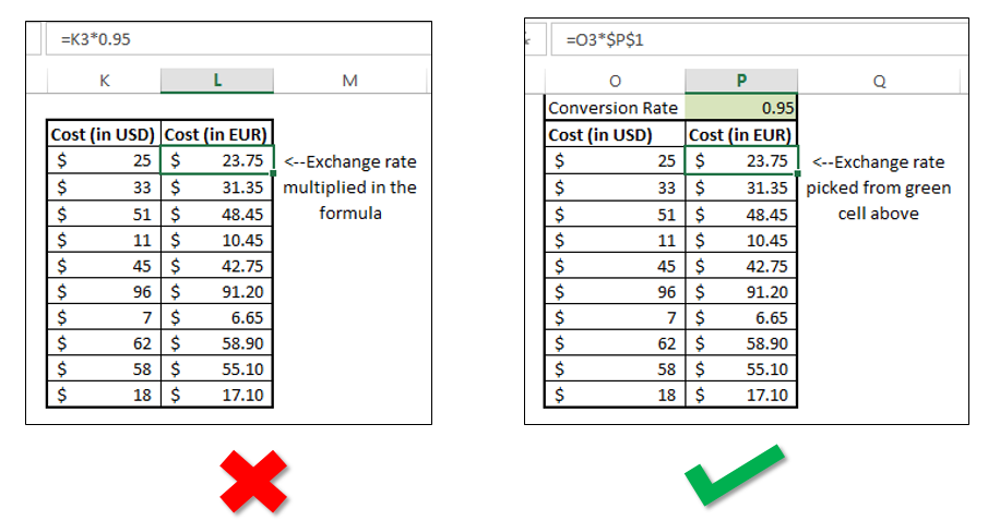
You can be the best thing that has happened to the mankind since sliced bread, but if you don’t have proper skills to make sense of the data you might as well be a potato sitting on your boss’s chair.

(Don’t you love it when someone strings random analogies together and yet it sounds logical?)

With the explosion of data capture technologies and focus on data-driven decision making, I often hear young professionals complaining of “too much data” and getting lost in the gigabytes upon gigabytes of ones and zeroes without truly being able to deliver insights from them.

In this series of articles, we’ll learn supply chain modeling for different types of supply chain problems. We’ll also learn how to present the data in a way it makes the most sense. And based on extensive experience with scores of the clients across the globe, I can safely state that this skill can easily catapult you in top 5% of supply chain professionals who just don’t solve problems reactively but solve them even before they become one.

Before we delve into specific situation-specific models and visualization for supply chain, let us take a moment to understand some basic principles of supply chain modeling. Spreadsheet models and cranky bosses have a tendency to go out of hand pretty soon, and messy excel sheets can only exacerbate the situation. These basic tips and approaches will go a long way in keeping your thought process structured and your bosses calm.

First, let us start with a hypothetical supply chain problem and following it through.

Long time ago in a galaxy far, far away...you worked for an organization that manufactures lightsabers, walkers, droids and other necessary stuff for the Galactic Empire.

Your boss, who works under someone who works under someone who works under Darth Vader himself, has tasked you with calculating the warehousing space the Empire would need in five years time. It’s now up to you, dear SCD, to find the answers the dark lord seeks to help him defeat the rebel forces.

Your heart stops beating for a second as you hear your boss give you this hopelessly daunting task. Not only you know next to nothing about organization’s growth plans, the sheer number of variables makes your head spin. You take a deep breath and stare at the blank excel sheet staring back at you.

Step 1: Clearly identify the objective of your model

Shut-down the lid of your laptop and first pick-up a pen and paper. Close your eyes and reflect for a moment what is really asked of you. Now write it down. You write the following:

Objective: To assess the warehousing space needed by your organization for the next 5 years

Now look long and hard at the objective you have written. Is this complete? Will your boss be happy with this output or he is looking for something more that he doesn’t know yet?

Aha! You strike-out what you had written and re-write the objective -

Objective: To assess the warehousing space needed by your organization for the next 5 years

Objective: To assess the warehousing space needed by your organization by region for the next 5 years

If you don’t get the objective right, chances are that you would be answering the wrong question all the while. Secondly, stating the objective clearly now saves a lot of re-work later. For e.g. had you just given your boss country level warehousing numbers, the immediate next question would be – “Well, how much of that is in the north?” and you’d have to come back to square one because you never thought to get that additional info in your model.

Step 2: Identify key inputs

Don’t open that distracting laptop yet. Next key step is to think through all inputs that you’d need to achieve your objective in step 1. Don’t worry about how or where you’ll get the data or information yet. Just think.

You sigh as your head fills with protesting voices. “This is so hopeless...how am I going to achieve this objective...I mean I don’t even know how much we are going to sell in 5 years...Aha!

You get that first item on your list of inputs:

1. Five-year forecast by region

B...But...there are several departments and all of them have different growth plans. Perhaps I need to approach them individually for their forecasts.Hmmm.

1. Five-year forecast by region and department

You take the logic further:

If I knew how many boxes each of the departments will sell and then multiply that by area each of the boxes will occupy...

2.Product Master including packaging sizes

Very Soon, by following your logic till the end, you arrive at this list:


1. Five-year forecast by region and department

2. Product Master including packaging sizes

3. No of items that come in a box

4. Stacking norms by the product

5. Inventory turns by product (by region?)

6. Other space requirements in the warehouse (e.g. aisle space)


Again - don’t worry too much if you don’t list each and every one of the inputs. When you start modeling, you’ll notice your requirements more closely.

Step 3: Build Input Sheets

Alright, open your laptop now. Answer those umpteen messages and mails; we’ll wait right here. Done? Good. Now open a blank excel sheet and create few tabs for the inputs. It’s a good idea to group similar inputs together in one tab.

No Empire can survive without Potato Chips inputs-forecast

inputs-supply-chain

Download the file here.

Put some dummy data in the blanks just so that you get the number formatting right and you’ll get some sensible values when you put some formulas in there.

We’ll a have separate post on these little tips and tricks of modeling.

Step 4: Create an output sheet and put formulas

It’s always better to create a separate output sheet. That way you can keep your calculations and data processing separated from your data. If there are multiple steps in the output, create intermediate output sheets too. Since, our warehousing problem in relatively simple, we’ll just have one.

And now the most difficult part – put formulas in your output sheet that can combine all the inputs together. Few tips:

1.Don’t be scared to create multiple tabs or multiple tables in your output tab if there are multiple steps involved.

2.You may also need to restructure your tables to see which one is most efficient with the formula. g. Should I put years in rows or columns? Will it create problems for me while dragging the formula across?

3.Create formulas and voila! You have your 5-year projection of warehousing space by the region.

Download the file with the output here.

Step 5: Present the data

If you showed this output to your boss, he’ll stare at the heap of numbers that you have calculated, might pretend to understand it and forget all about it till the last possible moment.

output

Your numbers are, of course, correct, but they don’t tell a story. There are no insights from the numbers you have churned so meticulously. Not only your boss but any of the stakeholders will require you to sit with them to explain these numbers. Your work should be able to stand on its own and shouldn’t need a theoretical physicist to understand it.

That’s where data visualization and dashboarding comes into the picture. It takes the data that only you understand and converts it into a super powerful decision enabling tool for EVERYONE. Don’t believe us? Here is the same data presented in a better way.

dashboard


Download the file with the Dashboard here. (You may be prompted to enable editing in order to use the sliders and check-boxes on the dashboard.)

This tells a story – on the left-hand side map, you can clearly visualize year on year increment of warehousing area by region along with current capacities, on the right-hand side you see the breakdown of area requirement by the department. You can even custom select the departments for easy comparison. To top it off, in the middle, we have the basic information about overall area required in a cool slot machine animation.

And that is not it. For even more inquisitive and demanding bosses, who want to tweak some inputs (c’mon SCD, we will improve on our inventory turns next year), there are hyperlinks to the relevant sheets at the bottom-right where they can tweak the inputs and the dashboard will be updated automatically.

We will have a separate article on dashboarding; meanwhile go ahead and play with the warehousing model that you have created from scratch in 5 easy steps.

This is bound to get your boss’s eyes widened and get your name resounding in the mighty boardrooms and corner offices. Welcome to the club, SCD.

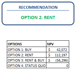
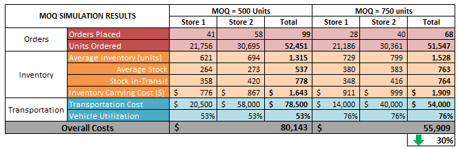
This is one of the most contentious questions that is often raised in review meetings especially during months of high inventory. We’ve all been there - where all the inventory indicators are in red, warehouses are overflowing with stuff, several leaning Towers of Pisa in the DCs are a common sight and trucks are waiting for hours to unload their stuff. The supply chain VP’s phone is ringing non-stop and when it seems that nothing can go worse, you suddenly realize that you have an S&OP meeting to attend to.

As you expected, the meeting is a bloodbath - S&OP chair, with deep burrows on his face, points finger at supply chain, others join in. Supply chain, on the other hand, blames faulty forecasting numbers. Demand planning, in turn, blames the inputs especially the sales projections; and when confronted, sales talks about their top-down targets and narrate in vivid detail how they didn’t receive right marketing support and how Supply Chain didn’t ensure that inventory was at the right place at the right time, thus completing the full circle of shrugging the responsibility of inventory ownership.

To muddy the waters even further, that one person from finance mumbles how “Inventory” is on the asset side of the balance sheet1 but still recommending to reduce it as the cost of borrowing is getting higher.

So, who is responsible for the inventory after all?

As the norm has become with this blog, the answer is – “Well, it’s more complicated than that.”

You see, inventory is not a single homogenous bloc that can be assigned or attributed to a single department or function, but a culmination of several direct and indirect causes across the organization.

In fact, Harold S. Geneen, has famously said, apart from his many other famous quotes,

All the problems of business end up in inventory


That’s true. Isn’t it?

Bad forecasting accuracy? – you’ll end up with unsold stock in inventory

Quality problems? – you’ll end up with returns in inventory

Bad roads? – you’ll end with damaged stock in inventory

Failed new product launch? – you’ll end with dead stock in inventory

Bad customer service? – you’ll end with canceled orders and... you guessed it, inventory

Very high customer service? – you’ll need to maintain high safety stock which is...inventory

So, are we doomed to live with this inventory mess forever without figuring out the real culprits? Is there no one who can save us from this impending inventory apocalypse?

Cool down, cut down on dramatics and dial a supply chain detective.

The solution to this mess is actually quite simple. A quick word of advice for SCZs out there – whenever you come across what seems like an insurmountable problem and you are unable to make a headway, start breaking the problem into its individual pieces, trace them back to their source and treat them individually. Once you solve the pieces, put them back together and voila – you have a solution.

For inventory ownership, the problem may look unassailable but let’s start breaking it. The good news is that we already know some of the inventory components. See! The moment we said inventory components, you’d know what is about to come already.

Cycle Stock

The first and often the biggest component of inventory is Cycle stock. It is the inventory that is needed to fulfill the average customer demand between the orders. Simply put, it is all the stock that is meant for selling before you receive the next inbound.

Cycle stock is dependent on two factors = Annual Demand and Inventory turns2.

While annual demand is an independent variable, inventory turns (the ability to churn your inventory) is something that is inherent in organizational strategy which in turn impact supply chain design and policies3 around it.

Let’s take an example –imagine there are two organizations named SavingPrivatePenny Inc (SPP) and FastAndFurious (FAF) Inc. SPP focuses a lot on cost efficiencies while FAF tries to be more responsive to their customers. With these different high-level strategies, SPP has a supply chain policy that prohibits less than 80% FTL load to be shipped. FAF Inc. Doesn’t have such policies and their trucks often go half unutilized.

In this example, SPP will have lower inventory turns vs FAF Inc. By extension – SPP will have higher cycle stock than FAF due to a. Organizational Strategy b. Supply Chain design.

[Some professionals blindly assume that SPP is a better organization than FAF. We’ll discuss this in another article why it’s a wrong pre-assumption without proper assessment.]

In a nutshell, cycle stock seems to be the responsibility of SCM function. However, supply chain design which has set a lower bound on cycle stock, also depends on financial constraints and overall organizational strategy.

Safety Stock

Demand-supply fluctuations are the name of the game and safety stock is the secret weapon in the arsenal of the organization that can help maintain the desired service level despite these fluctuations. However, this weapon comes at a cost. And that cost is inventory in form of safety stock. Higher the target service level, higher is the safety stock you need that may or may not be used that leads to higher inventory. In fact, the service level is the only deciding factor in determining the safety stock.4  

So who owns the safety stock?

Simple. Whoever decides on the service levels. In most cases, this is something that is defined by Strategy (since they define the market positioning of the organization) and Sales (as they back-feed the strategy on customer requirements). But it varies widely from organization to organization.

Hence, safety stock inventory component is something that should be owned by strategy or sales. (Or whosoever is taking call on the service level).

Other Miscellaneous Inventory

You’ll notice that even after accounting for cycle stock and safety stock, you’re left with unaccounted inventory. This is something that is often reported as “Excess Inventory”. It is a curious mix of different types of stock that ends up in excess inventory bucket.

Unsaleable Stock: This one is my personal favorite. It consists of all kinds of expired, damaged or otherwise unsaleable stock. The reason this is my favorite is that more often than not this represents a good percentage of overall inventory. And it’s relatively easy to get rid of – you have to simply write it off.

The expired products are due to over-forecasting, and that ownership needs to be shared between the businesses and the demand planning. Damages fall right on SCM and should hit their KPIs.

Interestingly, most of the organizations are aware of this bucket but they don’t want to do the write-offs. Why? Remember when we said at the beginning that inventory is treated like an asset on the balance sheet. Well, write-offs of this inventory, that could be valued millions of dollars on the balance sheet, forces the company to take a huge one-time loss that could be detrimental to its share prices.

This hesitation is natural since no CEO wants to take this dent on the share prices and on his/her bonuses. But keeping this bad stock not only reduces its salvage value but also eats up valuable warehousing space. So, a good SCD must always push for continuously identifying and reducing this unsaleable stock from their supply chains.

This problem was quite visible in the banking industry (Surprise! You can apply SCM concepts to the banking industry too!) in 2008-09 where banking behemoths refused to identify their own toxic assets leading to the biggest global meltdown the world had ever seen since the great depression.

Bonus question: What is “inventory” in banking context? Does EOQ formula hold any significance in such context? What does ‘quantity’ in Economic Order Quantity refers to?

QC Stock: The stock under quality check can be quite significant especially for high-value items or high-tech industry where the quality process can take several days. The ownership of this stock is with Quality, Manufacturing or procurement depending upon your organization. Being in QC doesn’t mean that this inventory can not be reduced. We’ll have an entire post detailing inventory reduction

Promotional Stock: Remember that promotion scheme when you gave out Boyfriend Pillow to your customers for free – when your customers looked long and hard at you wondering if they should be seen in the vicinity of your products; and where, even after six-months of trying to push it down the throat of unsuspecting customers, dealers, wholesalers and mortal enemies, there are still mountains of this abomination lying somewhere in the corner of your warehouse.Yeah, that one.

Dispose it off and put it on marketing’s account. Done.

Blocked Stock: All ERP systems offer stock blocking to prevent multiple sales commitments on the same stock. Once the stock is “blocked” it is unavailable for committing to another customer. However, this functionality is sometimes used to game the system to hoard the stock even for tentative sales. We’ll see various means by which this can be reduced but one thing is clear that the ownership of this inventory lies with the sales.


In conclusion, I want to reiterate that high inventory can be a real big pain for the organizations as it locks up capital, occupies valuable warehousing space and chokes us the free movement of stock though the supply chain. Identification of its ownership goes a long way towards taking the corrective action because if you don’t know who owns it, you will never know how to fix it.

This ownership should be built directly into the KPIs to ensure that right action is taken at the right time.

Do you have something to ask or say about inventory ownership? Please let us know through your comments.


Footnotes:

1 It is important to note that balance sheet inventory also includes raw material and WIP inventory. However, in the current article, we are focusing on FG inventory.

2 Hardcore SCDs might argue that the equation is other way round, where inventory turns is calculated from average inventory and COGS. Secondly, average inventory and cycle stock are two different things as former also includes safety stock and other misc inventory like returns, damaged good etc.

While these arguments are correct, in this article’s context we are looking at inventory turns more from a network capability viewpoint and not as a performance metric.

3 If your policies aren’t centered around overall supply chain design and organizational strategy, your supply chain goals will always be in conflict with the organizational goals. For e.g. If you claim to be a super-responsive pizza delivery chain, then your supply chain’s goal can’t be vehicle utilization. You’d have to be prepared for small orders that need to be delivered in 30 mins even if it means carrying one pizza in one van.

4 All other variables in safety stock calculation are not directly controllable e.g. demand variability, Lead Time etc.

Hello Detectives!

Now that you’ve learned the EOQ and its complex variations in part 1 and part 2 of this article, you are ready to use your new super power and save millions of dollars for your company. But before you knock on the corner office of your CEO or Supply Chain VP, be prepared to answer some questions that will be thrown your way.
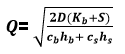
[At this juncture, some of you might be feeling that we are splitting hairs on EOQ formula. Do yourself a favor and do a back of the envelope calculation on how much total cost changes just by changing the ordering quantity 2% on either side. Total cost swings a lot, even for tiny changes in the ordering quantity.]

Complication #1: Your EOQ is not your supplier’s EOQ
Alright, so you’ve created fancy versions of EOQ models, gathered data on ordering cost and carrying cost through hook or crook, done tons of calculations, and checked and rechecked your numbers. And to your delight, it looks perfect. Not only that, it seems that implementing new EOQ numbers will save a few million dollars for your company every year. But just when it seems that there is nothing between you and that Employee of the Year award, your order is rejected by...the supplier.

But why? Simple. Your order quantity might be the best thing that has ever happened to your organization, it is not feasible for the supplier to manufacture. Supplier has his own manufacturing processes, its own suppliers and his own optimal batch sizes, and the order quantity you are demanding isn’t financially viable for him. For example, remember when we calculated the EOQ of 20 in previous illustration earlier. But what if supplier’s batch run produces only 15 units at a time. This means that he’ll have to run two batches of production to produce 30 units and after fulfilling your “optimal” order of 20, sit on remaining 10 units waiting for your next order. The problem is even worse if his batch size is, say, 50 units.

Well, there are two ways out of the situation – the easy way, where you arm-twist the supplier to your will and push him to absorb the loss which is the most common practice in such situations but in long term results in supplier mistrust, higher inventory at the supplier, and maybe renegotiation of the whole contract.

The slightly difficult way –that will ensure more transparency, collaboration and even bigger savings than the EOQ formula - is called Joint EOQ formula.
[Also known as Joint Economic Lot Size (JELS) formula]

The underlying principle behind Joint EOQ is pretty simple as you might have guessed from its name – it tries to find an optimal EOQ for the supplier-buyer system considered as one. Imagine if supplier was part of your organization – in that case how would you calculate the optimal order quantitiy that needs to be produced.

Let us re-write our total cost equation

Total Cost = Ordering Cost (for both supplier and buyer)+ Carrying cost (for both supplier and buyer)

jels-1
Where, D is annual demand
Q is the order quantity
Kb is the Ordering cost for the buyer
S is the set-up cost for the supplier
hb, hs Inventory carrying cost for buyer and supplier respectively
cb, cs purchasing cost for buyer and supplier respectively.
We repeat the same procedure of differentiating both the sides by dQ and solve for Q.

jels-2

The beauty of this JELS quantity is that is leads to even lower cost than what buyer and supplier could have individually achieved. THAT is the power of collaboration right there.

Bonus question: What are the total savings for supplier and buyer combined by moving to JELS than their individual optimal quantities? What should be a fair split of benefits between them?
[For a detailed read on JELS you may want to read this famous paper. Please note that the notations used in the paper are slightly different.]

Complication #2: FTL ≠ EOQ
If you pay your logistics provide by the unit then don’t read further. You can merrily start implementing EOQs and punching those 1 unit orders.

However, if you pay your logistics provider by the trip or the route, you’d notice that EOQ quantities may lead to lower utilization of your vehicles. And since you pay for the whole vehicle whether it has one unit inside it or one hundred, you lose some money on every trip when you order EOQ.

Solution:
First check whether there are “right-sized” vehicles available with your logistics service provider. Your ideal situation is where EOQ matches exactly with the vehicle capacity.

If EOQ doesn’t align with the vehicle capacity, compare the total cost between partially filled vehicle (LTL) and FTL vehicle. When vehicle is FTL you end up increasing your inventory. It might still be worthwhile to under-utilize the vehicle.

[There are modified EOQ models available where transportation costs are taken as a step function.]
Multi-product ordering : If the supplier deals in multiple products, explore an option to combine multiple products in the same order.

Supplier clustering and multi-pick ups: If there are other suppliers in the vicinity, you may want to club your other orders in the same vehicle. This can also be implemented at buyer’s end where multiple buyers of the same suppliers combine their orders for better efficiencies.

This strategy to maximize vehicle utilization, albeit without EOQ reasons, is quite a common practice for non-competing organizations. Best example, perhaps, is where Nirma sent its heavy detergent packets inside Sintex’s empty water tanks to maximize the vehicle utilization leading to the savings for both the organizations.

Vehicle utilization and idle time reduction is an area of prime focus for the organizations with lot of resources and effort going into improving it. Hence, there will be whole another post to discuss it in detail.

Complication #3: Warehouse Capacities
At times, especially when pushed by deep discounts from the suppliers, EOQ formula may recommend huge buys. However, warehouse capacities are not infinite and handling additional inventory may require additional manpower, equipment or space.

Solution:
In such rare cases, it is useful to consider warehousing costs as increasing with inventory. This is something we tackled in part 2 where we considered inventory carrying costs to be a function of quantity.

Closing Remarks
Phew! That was a long read. But I hope that has you transformed from a Supply Chain Zombie (SCZ) who used to take orders from bosses and the clients to a Supply Chain Detective (SCD) who doesn’t rely on “thumb rules” and “common practices”.

In fact, the aim of this article wasn’t to cover each and every possible scenario in the book and churn out dozens of formulas but arm you with the thought process and the techniques to handle all sorts of complicated situations that might come your way. If I’ve succeeded in this attempt, do let us know through your comments.

Go ahead, now, change the world.