Hello Detectives!

Now that you’ve learned the EOQ and its complex variations in part 1 and part 2 of this article, you are ready to use your new super power and save millions of dollars for your company. But before you knock on the corner office of your CEO or Supply Chain VP, be prepared to answer some questions that will be thrown your way.

[At this juncture, some of you might be feeling that we are splitting hairs on EOQ formula. Do yourself a favor and do a back of the envelope calculation on how much total cost changes just by changing the ordering quantity 2% on either side. Total cost swings a lot, even for tiny changes in the ordering quantity.]

Complication #1: Your EOQ is not your supplier’s EOQ
Alright, so you’ve created fancy versions of EOQ models, gathered data on ordering cost and carrying cost through hook or crook, done tons of calculations, and checked and rechecked your numbers. And to your delight, it looks perfect. Not only that, it seems that implementing new EOQ numbers will save a few million dollars for your company every year. But just when it seems that there is nothing between you and that Employee of the Year award, your order is rejected by...the supplier.

But why? Simple. Your order quantity might be the best thing that has ever happened to your organization, it is not feasible for the supplier to manufacture. Supplier has his own manufacturing processes, its own suppliers and his own optimal batch sizes, and the order quantity you are demanding isn’t financially viable for him. For example, remember when we calculated the EOQ of 20 in previous illustration earlier. But what if supplier’s batch run produces only 15 units at a time. This means that he’ll have to run two batches of production to produce 30 units and after fulfilling your “optimal” order of 20, sit on remaining 10 units waiting for your next order. The problem is even worse if his batch size is, say, 50 units.

Well, there are two ways out of the situation – the easy way, where you arm-twist the supplier to your will and push him to absorb the loss which is the most common practice in such situations but in long term results in supplier mistrust, higher inventory at the supplier, and maybe renegotiation of the whole contract.

The slightly difficult way –that will ensure more transparency, collaboration and even bigger savings than the EOQ formula - is called Joint EOQ formula.
[Also known as Joint Economic Lot Size (JELS) formula]

The underlying principle behind Joint EOQ is pretty simple as you might have guessed from its name – it tries to find an optimal EOQ for the supplier-buyer system considered as one. Imagine if supplier was part of your organization – in that case how would you calculate the optimal order quantitiy that needs to be produced.

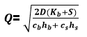
Let us re-write our total cost equation

Total Cost = Ordering Cost (for both supplier and buyer)+ Carrying cost (for both supplier and buyer)

Where, D is annual demand
Q is the order quantity
Kb is the Ordering cost for the buyer
S is the set-up cost for the supplier
hb, hs Inventory carrying cost for buyer and supplier respectively
cb, cs purchasing cost for buyer and supplier respectively.
We repeat the same procedure of differentiating both the sides by dQ and solve for Q.

The beauty of this JELS quantity is that is leads to even lower cost than what buyer and supplier could have individually achieved. THAT is the power of collaboration right there.

Bonus question: What are the total savings for supplier and buyer combined by moving to JELS than their individual optimal quantities? What should be a fair split of benefits between them?
[For a detailed read on JELS you may want to read this famous paper. Please note that the notations used in the paper are slightly different.]

Complication #2: FTL ≠ EOQ
If you pay your logistics provide by the unit then don’t read further. You can merrily start implementing EOQs and punching those 1 unit orders.

However, if you pay your logistics provider by the trip or the route, you’d notice that EOQ quantities may lead to lower utilization of your vehicles. And since you pay for the whole vehicle whether it has one unit inside it or one hundred, you lose some money on every trip when you order EOQ.

Solution:
First check whether there are “right-sized” vehicles available with your logistics service provider. Your ideal situation is where EOQ matches exactly with the vehicle capacity.

If EOQ doesn’t align with the vehicle capacity, compare the total cost between partially filled vehicle (LTL) and FTL vehicle. When vehicle is FTL you end up increasing your inventory. It might still be worthwhile to under-utilize the vehicle.

[There are modified EOQ models available where transportation costs are taken as a step function.]
Multi-product ordering : If the supplier deals in multiple products, explore an option to combine multiple products in the same order.

Supplier clustering and multi-pick ups: If there are other suppliers in the vicinity, you may want to club your other orders in the same vehicle. This can also be implemented at buyer’s end where multiple buyers of the same suppliers combine their orders for better efficiencies.

This strategy to maximize vehicle utilization, albeit without EOQ reasons, is quite a common practice for non-competing organizations. Best example, perhaps, is where Nirma sent its heavy detergent packets inside Sintex’s empty water tanks to maximize the vehicle utilization leading to the savings for both the organizations.

Vehicle utilization and idle time reduction is an area of prime focus for the organizations with lot of resources and effort going into improving it. Hence, there will be whole another post to discuss it in detail.

Complication #3: Warehouse Capacities
At times, especially when pushed by deep discounts from the suppliers, EOQ formula may recommend huge buys. However, warehouse capacities are not infinite and handling additional inventory may require additional manpower, equipment or space.

Solution:
In such rare cases, it is useful to consider warehousing costs as increasing with inventory. This is something we tackled in part 2 where we considered inventory carrying costs to be a function of quantity.

Closing Remarks
Phew! That was a long read. But I hope that has you transformed from a Supply Chain Zombie (SCZ) who used to take orders from bosses and the clients to a Supply Chain Detective (SCD) who doesn’t rely on “thumb rules” and “common practices”.

In fact, the aim of this article wasn’t to cover each and every possible scenario in the book and churn out dozens of formulas but arm you with the thought process and the techniques to handle all sorts of complicated situations that might come your way. If I’ve succeeded in this attempt, do let us know through your comments.

Go ahead, now, change the world.