Life is replete with trade-offs. Whenever we take any decision we have to think about all positives and negatives.
Shall I live closer to the city to save on commute OR live on the countryside to save on rent?
Shall I buy a smaller quantity to save on my inventory costs OR buy in bulk to save on ordering costs?
Shall I marry the girl who is more beautiful and rich OR the one who is more intelligent, empathetic and caring?
While the last trade-off can’t be evaluated by Excel modeling...
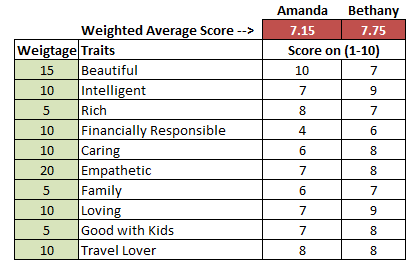
...never mind.
Whatever is the problem, we have to evaluate trade-offs involved to arrive at the most reasonable answer. An optimized answer.
There is tons of theory that goes behind Linear Programming and optimization, but this SCD thinks that best way to understand the concept is through a story. And what better story than one that is worth $ 42 billion.
PROBLEM

Han Solo and Chewbacca, smugglers in a galaxy far far away, while trying to dodge the troublesome Imperial law enforcement, have landed their famous spaceship the Millennium Falcon on an unknown planet called Excel –XIII. While searching for a good place to go underground, they encounter a trader who is selling some interesting stuff at a good bargain.
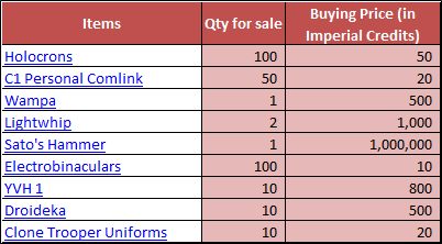
However, there are some big constraints because of which he can’t buy everything on offer.
Han Solo, never to miss out on a good money making proposition, realizes that he can make a profit on all the items listed above with the trader.
1.His spaceship doesn’t have space for everything (he only has 20,000 cubic cm)
2.He doesn’t have enough money to buy everything (he only has 10,000 credits)
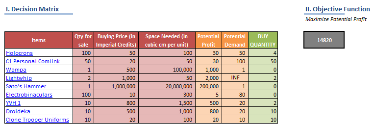
Being a shrewd smuggler and a businessman that he is, his objective is to optimize this deal and maximize his profit. He quickly adds more information to the table:
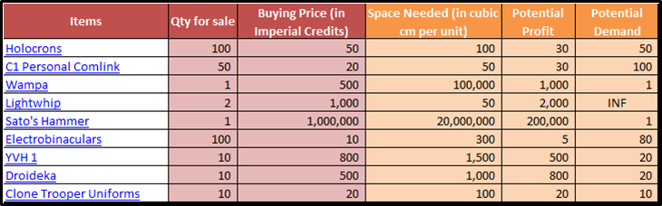
As we can see above he has added three more columns
Space requirement – that tells us how much space is needed for each unit of the item
Potential profit – that tells us how much profit Han Solo stands to earn by selling that item elsewhere and,
Potential demand – that tells us how much quantity of that item that Han should be able to sell
He realizes that manually figuring out what items he should buy and in what quantity would be a mammoth task that’d take him a long time. Fortunately, he is on the planet of Excel-XIII where he has the right tools at his disposal. With Chewbacca's help, he decides to build an Excel based optimization model.
Download the file with the model.
Han knows three steps for modeling any optimization problem. So, he jots down the following:
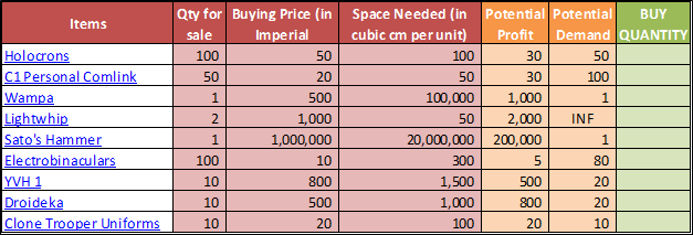
Step 1: Identify the decision variables
Decision variables are simply the things we want to solve for. For e.g. Han wants to know which items he should buy in what quantity.
He the adds another column to the table, called “Buy Quantity”. He doesn’t know the values yet so those values remain blank. In fact, he wants the magic of optimization to fill in these cells for him.
Step 2: Write the objective function
Objective is nothing but the ultimate goal we are trying to achieve. Maximising profit, minimizing the cost, maximizing the score in our girl selection problem are some examples of objectives.
For Han, it is to maximize his profit from the proposed trade.
When objective is represented mathematically it becomes an objective function. E.g. Sales x margin, production x cost etc. are the examples of objective function
Han puts a formula in the cell that calculates his profit. This is the sum of profit from the all the items that he is planning to buy. Though there is a formula there, the value in the cell is zero since there are no values in the “Buy Quantity” column that it uses as one of the input.
Step 3: Identify the constraints
Han would’ve bought everything had there weren’t any constraints. But sadly he does:
Constraint 1: His spaceship doesn’t have space for everything. He has only 20,000 cu cm.
Constraint 2: He doesn’t have enough money to buy everything. He has only 10,000 credits.
Apart from these explicit constraints, there are some hidden constraints that you simply know from common sense but we have to explicitly tell the computer. Remember that famous adage from the 1990’s that said: “Computer is loyal but foolish servant”.
Constraint 3: Han can’t buy more than what is available with the trader.
Constraint 4: Han can’t (or rather shouldn’t) buy more than what he can sell.
Constraint 5: Buying quantities can’t be negative.
Constraint 6: Buying quantities have to be an integer.
Solver Set-up
Alright, so you have successfully set-up the whole model. You’d be happy to hear that that was the toughest part of optimization. Now, you have to just run - something very appropriately called - “Solver”, that will evaluate these trade-offs, work under the constraints and optimize the objective by changing the decision variables.
But first, where is this magic called “Solver” you might ask. Don’t worry – “Solver” add-in comes free with all excel and you can find it under the Data tab.

If you don’t see it just head down to File --> Options --> Add-Ins --> Manage --> Select “Excel Add-ins” from the drop down --> Go --> Check the box “Solver Add-In”
When you click on “Solver”, you’ll get the following pop-up box.
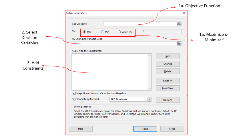
Now we have to tell the solver about our decision variables, objective function, and the constraints. We strongly recommend that you try to model alongside using the model you just downloaded.
Step 1: Set Objective
 Step 2. Select decision variables
 Step 3. Add Constraints
 Step 4. RUN!
This is the most fun part where you click solve and see the Solver run through several decision variables. Download the file with optimized values here.
Voila! Han has the optimized quantity he must buy for each of the items. His profit will be 14,280 which is a great return on his original investment of 10,000.
We can also see that he is running out of money rather than space. Hence, money constraint (Constraint#2) is called a limiting constraint while space is a non-limiting constraint.
Take your time with the model and experiment with it. Change the constraints; tweak the objective function or try to relax a few constraints and observe how it changes the results. Try to think the problems for which this can apply to your organization. Analyze the solution reports.
CONCLUSION
Supply Chain Management is all about trade-offs – be it high stakes network optimization problems, tricky buy vs source decisions or cumbersome manufacturing line allocations – LP modeling and solver is one of the most powerful tools a supply chain professional can have at his disposal. In fact, the moment you’ve practiced a few problems, you’ll find its applications literally everywhere. Therefore, it can’t be over-emphasized that an expertise in LP modeling makes the difference between a Supply Chain Zombie and an awesome SCD.