Author: admin

Good to see that you have made to part-II of this article. If you have not done so yet, I strongly recommend you to check-out the first part where we derived this deceptively simple EOQ formula.
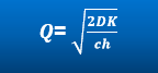
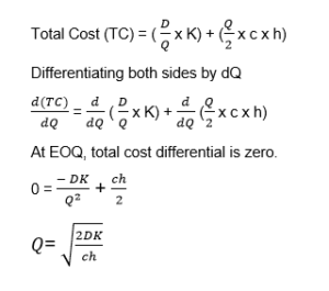
eoq-formula

Where,

Q is Economic Order Quantity

D is Annual demand (in units)

K is Ordering Cost (in $) per order

c is Cost of the product (in $ per unit) and,

h is the inventory carrying cost (as %age of product cost, incurred annually)

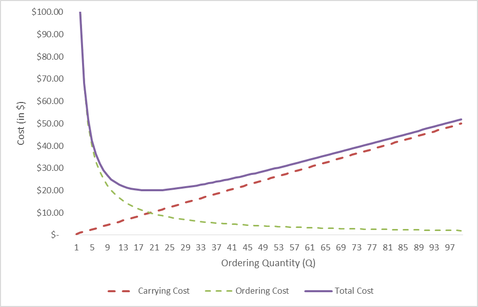
In this post we’ll see why EOQ formula should be rarely used in its basic form. And even if you were to use it, you must at least be aware of the caveats and assumptions that have gone into it.

We’ll do that in two parts. First let us challenge some assumptions that we made earlier and then we’ll put in some real world complications that require us to tweak the formula or add in some layers of analysis before we start using the order quantity recommendations.

Assumption #1: Inventory Depletion is uniform

One of the major assumption while deriving the formula was uniform inventory consumption. And that is how we arrived at Q/2 as average inventory. However, this is seldom true. Rate of consumption changes from season to season, week to week and even day to day.

Solution: An ideal solution is to come up with a consumption curve (Inventory vs Time graph) and use it to calculate average inventory over time. However, this may involve doing an integral of a complex curve. If you want to be super-precise then that’d the way to go but there are more practical and easier approximations to this problem that will give you “good” solutions with a lot less effort.

Approximation: Rather than one continuous curve, we can break our time period into two or more sub-periods each having a simpler consumption pattern. For example,  a vast majority of FMCG organizations make most of their sales during the last week of the month. This could be a typical case of student syndrome where sales team is pushing to meet their monthly targets. [This takes a significant toll on supply chain infrastructure and many organizations struggle to manage these last week peaks. We will dedicate a separate post to this topic.]

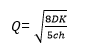
So, let us say that 50% of the monthly demand is consumed in first three weeks while remaining 50% is consumed in last week itself. In other words, consumption rate during last week is thrice that of first three weeks. Over long-term1, the average inventory can be calculated to be 5Q/8. We leave it to the readers to derive this number. You may notice that this average inventory is higher than (Q/2) that we calculated earlier where the inventory depletion was uniform throughout. This makes sense as earlier we had consumed 75% of the monthly demand in 3 weeks whereas we have only consumed 50% in the current scenario, leaving us with slightly higher inventory.

If we put 5Q/8 as average inventory in Total cost equation:

eoq-part-2-modified-eoq

We can derive modified EOQ as:

eoq-part-2-modified-eoqb

Similarly, now you can derive your own EOQ formula given any consumption rate or consumption pattern.

Assumption #2: Cost of the material is constant regardless of quantity

Remember when we wrote the total cost equation as

total-cost

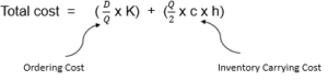
We deliberately didn’t consider one element of cost in the above equation which was buying cost. We ignored it because it wasn’t relevant as we were spending the same amount annually despite of ordering quantity.

However, this assumption doesn’t hold true especially when buying quantities are large. Suppliers often provide bulk discount options as they save on producing at a scale. In fact a typical supplier quote looks like this:

QTY

1-20

21-50

51-100

101-150

151+

Price (per)

$ 5

$ 4.75

$ 4.5

$ 4.25

$ 4

As the quantity increases our buying cost decreases significantly. In fact supplier is willing to offer 20% discount if we buy more than 150 units of the product. But is it worth it?

Now, let us rewrite the total cost equation, this time around we’ll have to include the buying cost as it has become relevant.

total-cost-with-bulk-discounts

The product price c* is now a function of Q –

c* = $ 5 per unit (for Q between 1-20)

c* = $ 4.5 per unit (for Q between 21 -50)

...and so on.


Graphical Solution

Let us recreate the chart that we made earlier. This time around, we have an additional line for buying cost.

Download the workbook HERE.

Graph

As you can see in the graph above, buying cost is a step-curve. Those “steps” represent the bulk-discounts that supplier has offered. We also see these “steps” in total cost curve (the thick blue line) since it includes the buying cost. You’ll notice that now it is not so easy visually to find the minimum cost point on the total cost curve.

I checked the table that was used to create the graph in the workbook, and it turns out that minimum total cost is $ 461.7 while buying 151 units. Note that this is different from our non-discounted EOQ number where we got the answer as 20 units.

How will you sell this to the CEO? You can’t show derived EOQs and complex graphs, right? Well, you can simply state the following – “Usually, we should only buy 20 units at a time which is roughly one month of supply, however this time around the supplier is giving 20% discount on bulk orders. Sure, this increases our inventory costs a bit but it’ll be more than compensated by the discount.”

Interestingly, the next lowest cost $ 470 occurs at 101 units. So, if your CEO still frowns at you for asking to buy huge inventories, you can always fall back on the second best solution, where incurring 9 dollars extra reduces your inventory from 150 to 100.

[The second best or even third best solution may be more acceptable in some cases. True – that absolute minimum occurs at 151 units but just paying additional 9 dollars we can mitigate some of the unaccounted risks that come along with the additional inventory. This is a typical problem with all kinds of optimization algorithms. They try to reduce the objective function to the absolute minimum, a phenomenon that we describe as chasing the pennies. This is sometimes not desired. And this is where multi-objective optimization comes handy. However, that is another discussion for some other day.]

Analytical Solution

Above, we arrived at the solution by looking at the graph and corresponding data but that’s not feasible especially when large quantities are involved or we don’t have access to spreadsheet software.

While there is no straightforward formula for EOQ with bulk discount because buying cost is a step-function and hence non-differentiable, we still have a step-by-step procedure that can help us arrive at the best quantity.

Step 1: Find normal EOQ for ALL buying costs

In our example, there are five different costs. While we are not showing the detailed calculation their corresponding EOQ values are shown below. Subscript represents the cost(in $ per unit):

EOQ5       = 20 units

EOQ4.75  = 20.5 units

EOQ4.5    = 21.1 units

EOQ4.25  = 21.7 units

EOQ4      = 22.3 units

[Bonus Question: Keeping all the other factors constant, why does EOQ increases as the cost per unit decreases?]

Step 2: Eliminate “Invalid” solutions

Some of the EOQ quantities doesn’t belong to the buying cost. Eliminate them.

EOQ5       = 20 units

EOQ4.75  = 20.5 units X

EOQ4.5    = 21.1 units X

EOQ4.25  = 21.7 units X

EOQ4      = 22.3 units X

Note: You may be left with none or more than one solutions.

Step 3: Calculate and compare total costs for all the valid EOQ solutions and buying qty break-points

Qty Type

Qty (units)

Total Cost ($)

EOQ5

20

520

Bulk Qty 1

1

701.5

Bulk Qty 2

21

494.5

Bulk Qty 3

51

476.9

Bulk Qty 4

101

469.9

Bulk Qty 5

151

461.7

Total minimum cost is at Qty 151 which is our answer.

Assumption#3: Inventory Carrying Costs are constant

As briefly touched upon in previous part of this article, inventory carrying cost consists of several components – cost of capital (typically the borrowing rate of your organization), cost of storage (Warehousing costs and salaries) and cost of servicing the inventory (insurance, damages, obsolescence). Though it is highly organization dependent, finding the exact value might be a tricky task. It is usually taken between 17% and 25% depending the nature of the inventory and opportunity cost of capital to the organization.

However, some of these variables are not constant and vary with the quantity of inventory kept in the organization. Couple of examples are below:

Insurance cost: Per unit insurance cost decreases as average inventory increases.

Risk of damages/obsolescence: Risk of damages and obsolescence increases as average inventory increases.

Solution:

The solution requires some understanding of basic differentiation. If you don’t get it in the first attempt, don’t worry about it too much.

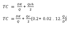
Let us say that by some measure of analytics, one has arrived on a inventory carrying cost equation

Inventory Carrying Cost (h)= r + f(Q)

h = 20% + 2%* [(Q/(D/12)]

Don’t get scared by the above equation. It simply states that inventory carrying cost is 20% plus 2% for addition of every month to order quantity. This 2% is attributed to the increasing risk because of incremental inventory. Hence for one month’s inventory, carrying cost = 22%, for two months its 24% and so on.

Putting this in the basic equation

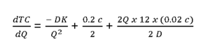
Differentiating both sides by dQ

For min TC,

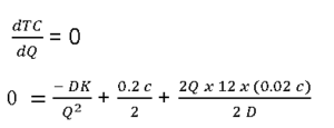
Simplifying the equation we get,

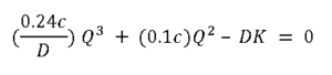
 Replacing the variable values, D = 100 units, c = $ 5, K = $2

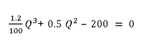
This is a cubic equation with three solutions for order quantity Q.

Q= 16.87, -29.2 ±11.44i

We can reject the complex solutions. Hence, the EOQ for dynamic carrying cost is ~ 17 units.

Note that this is slightly lower than our original solution of 20 units that considered fixed carrying cost of 20%. This seems logical as slight increase in carrying cost is reflected in decreased EOQ.

Conclusion

If you have reached this far, then CONGRATULATIONS! You’ve mastered the science behind ordering quantities and their trade-offs, you are now ready to take on any challenge that anyone in your organization can throw at you. Well, let me scratch that. You are almost ready.

There are some teeny-weeny complications that are often put to question your EOQ numbers. While some of those do not impact our EOQ too much, it is important to be aware of them to pave way for smooth implementation of your ideas. Part 3 of this article is dedicated to those complications and work-arounds.

[Boy, I never realized that this simple EOQ formula would take me 3 parts to finish. Well, grab some coffee and click on part 3]

Continue to part 3


Footnotes:

1 Order quantity may or may not be equal to one month’s demand. Hence, every month’s inventory profile will look different. E.g. if order quantity = 5 weeks, 1st month will see an ending inventory of 1 week, 2nd month will see ending inventory of 2 weeks and so on. Hence, we look at long term average of the inventory.

photo-1430760903787-4d91bbf15384If you asked any CEO, Sales Executive or Marketing head what is the customer service level they desire in the organization they’d invariably say 100%. And hearing that answer the Supply Chain VP will invariably shake their heads and flee the room before you could ask them the same question.

But why, you might ask, such an expectation is unreasonable for any organization in any industry? Intuitively, it seems alright to want to sell to anyone who is willing to pay you in crispy greens. In fact, primary purpose of existence of organization is shareholder value creation? Which in simple words mean that organizations solely exist to earn profit by selling their stuff. 

Before we delve deep – keep this thought at the back of your mind –

Organizations aim to maximize their profit

Let us try to understand this problem and define our problem statements more clearly.

1.Why it is unreasonable to have customer service level at 100%? And if it is, indeed, unreasonable then,

2.What is the optimum service level?

Qualitative Approach

Let us suppose you are the store manager in the said organization that sells consumer goods. You are responsible for managing stock on the shelves and ordering them before they go out of stock. Customer Service Level is your primary KPI and it is defined as percentage of times customer gets on the shelf whatever he is looking for.

Let us also imagine that one fine morning you get a memo from the CEO, the Sales VP and the marketing head (who must truly hate the supply chain guy) have decided to set this Customer Service Level as 100% as the new target.

Just yesterday you had to turn a guy back who wanted to buy five dozen television sets. With this new policy you’d have to stock everything that the next customer might need.

Oh heck, you realize that you need to stock your party supplies section for the next customer who accidentally invited 21,000 guests on her birthday. Even though the probability of this happening is very small, it is not zero. And the customer service target of 100% nudges you to be stocked for this small probability. Even if this means tons of overstocking and surely lot of wastage later, you have to be ready for all the extreme cases of demand.

You let out a muffled scream and consider quitting your job before sending a polite reply to your boss asking for permission to stock infinite inventory.

Quantitative Approach

We now intuitively understand why the customer service level can not be 100%. It would mean keeping infinite inventory for any possible customer demand that may or may not come. Keeping high inventory is almost sure to lead to excess inventory and write-offs ultimately making it a loss making proposition. But how much then should we “serve” before it starts becoming a loss making proposition.

Let us first take an example to understand the underlying logic before we go on to make complex models.

Imagine that you are that poor store manager responsible for customer service as well as inventory cost. The product that you sell costs $8 and you sell it at $20 for a net profit of $12. However, if you are unable to sell it, you’d incur a loss of $8 that was product cost.

The trade-off here is the profit that you’d earn if the customer walks in and you have it in your inventory

Vs

The loss that you’d incur if you stock and he doesn’t turn up.

So, should you buy the next unit  of inventory (it is very important to note that we are only talking about a single incremental unit) if there is only 25% chance that you’ll be able to sell it? What if this probability is 50%? 75%?

If the probability is 100%, that is you are sure to sell that next unit (I repeat, only one incremental unit) of product, then it’s a no-brainer that you’d want to stock it for a sure-shot profit of $12.

Now let’s take the next case where there is only 25% chance that you’ll sell it and make a profit of $12 but there is 75% chance that you won’t be able to sell it thereby incurring a loss of $8.

Your expected payoff from this extra inventory is = (25% x $12) + (75% x - $8)

= - $3

Since your expected payoff is negative when the probability is 25% , you’d not want to store this next unit of stock.

Similarly, the payoffs at 50% selling probability (Let’s call it P50 ) is  +$2 and at P75 is +$7

Let us summarize these results:

P25 = - $3

P50 = +$2

P75 = +$7

So, somewhere between 25% and 50% selling probability, keeping that extra unit in inventory became a profit making proposition. With little bit of maths we can find that probability is 40%

So, as long as probability of selling the next unit exceeds 40%, you’ll keep stocking the inventory.

40% looks like a pretty high number. In real life, you’ll find that organizations are willing to stock that extra unit, for far lower selling probabilities. There is a logical quantifiable reason behind this behavior even though a vast majority don't know about it. The reason is that profit on immediate sale ($12 in our case) is not the only gain you make from that customer. When a customer walks-in into your store and finds what he/she is looking for, he will continue coming to your store and give you all that future business. This value of all future goods that the customer would buy is called Customer Lifetime Value.

Continuing with the previous example, suppose Customer Lifetime Value at the above store is $100. i.e. if the customer keeps on coming to your store then you stand to profit $100 from that customer. However, if he doesn’t find the product he is looking for, he’ll take this business to your competitors. What is that selling probability at which you’ll keep that unit of inventory? Let’s call it S:

PS = (S x $100) + ((1-S) x -$8)

At the cut-off probability, payoff would be zero.

0 = 108S -100

S = 7%!

Surprising. 93% of the times you are not expecting to sell that one unit and yet you’ll keep it in store because in long run that one customer is going to pay-off by becoming your loyal customer.

So, in a nutshell, keeping extra inventory is determined by probability of us selling it for acquiring a customer lifetime value vs having to write-off the extra inventory.

Some of you might be wondering why we did this analysis for only one unit (and kept on harping upon the point repeatedly). This is because the probability of selling keeps on changing as you add more stock. The probability of selling the 1st unit is very different from probability of selling nth unit.

I’ll be bet my arm that a liquor store in the middle of alcoholic town will sell its first bottle during the first hour of the day. 50th bottle – maybe. 1000th bottle – all bets are off (because I love my arm way too much).

So, coming back to the original point, how do we do this analysis for all of stock and not just one unit? It is the next level of analysis of service level that deserves its own article. Keep tuned in - it'll be releasing soon.

All you supply chaiphoto-1431605695381-f4a9c3cdd150n zombies (SCZs), who are now vying for the blood of the crackpot who wrote such a blasphemy as the title of this post, take a deep breath, cool down a bit and think back at the time when you last implemented the EOQ formula in its basic form. That is – NEVER.

Hmmm...and now that you are thinking about it, doesn’t it seem strange that one of the most popular supply chain concepts and most widely recognized formula that is literally taught on the first day of supply chain classes in college, is rarely used in the real world?

Well, there is a solid reason behind it. Rather, reasons behind how the real world considerations make our basic EOQ formula difficult to use in practical situations.

And you can too traverse this journey from Supply Chain Zombie to the supply chain detectives by understanding these factors and then tweaking the formulas to make it more suitable for your organization’s context.

But before you scram to your boss to make him salivate with your $545 million formula and start planning o spend that six figure bonus that he’ll shower on you, lets first clear up our basics about EOQ.

For the seasoned Supply Chain Detectives, who understand the basics of EOQ inside out – feel free to skip to the second part of this article. For the rest of us lesser mortals– read on.

The Basic EOQ Formula

While your soporific professor mumbled something about carrying costs and ordering costs in Supply Chain 101 you dozed off while doodling aliens and space rockets in your notebook. Well, don’t worry, we’ve got you covered.

EOQ stands for Economic Order Quantity. Well, what does it mean?

Everyday billions of individuals and millions of organizations across the globe buy stuff. For individuals, it varies from buying eggs, bread & butter to 8 iPhones for a Dog.  And for organizations, it varies from manufacturing raw materials to office supplies, and from toilet papers to million dollar office decorations.

But, unless you are a billionaire owner of that Apple Watch brandishing dog, those billions of individuals and millions of organization must decide on one crucial factor while buying stuff – How much?

It may be intuitive for us to make the decision of ‘how much’ in some simple situations. E.g. eggs – On one hand you don’t want to buy too few eggs to save you trips to the grocery store everyday, one the other hand you also don’t want to buy too many to risk rotting them. And by using this rationale you settle on something in between say 1 week’s worth of supply.

What you are essentially doing here is trying to find a balance between two opposite cost elements – cost of visiting the grocery store too frequently vs cost of overstocking it.

This is what EOQ tells you. It finds the right balance between the Ordering Cost (cost of placing one order. In our example cost of visiting the grocery store once) and Carrying Cost (cost of carrying the inventory – storage costs, cost of capital etc.) mathematically and tells you exactly how much to buy.

Essentially what you are trying to minimize is the total cost of owning something.

Total Cost = Ordering Cost + Carrying Cost --- (1)

Let us look at both the components theoretically. Later in this article, we elaborate what actually constitutes ordering and carrying costs from the organization perspective. For now, we’ll stick to formulas.

Ordering Cost

Ordering Cost = Number of orders per year x Cost per order (K)

Number of orders per year = Annual demand (D) / Ordering Quantity (Q)

ordering-cost

Carrying Cost

Carrying Cost = Average Inventory (in $) over the year x Inventory Carrying Costs (h)

Average Inventory (in units) = (Q/2)

Average Inventory (in dollar) = (Q/2) x c

[Because we are ordering Q units at a time and it uniformly depletes to zero as the inventory is consumed. Hence, the average inventory is (Q+0)/2]

Carrying Cost = ( Q/2) x c x h

Let’s put back these numbers in total cost equation (1)

Total Cost (TC) = [( D/Q) x K] + [(Q/2) x c x h]

Now do you see why we need to find a sweet-spot of ordering quantity to minimize total costs? No?

Alright, pay close attention to the Q in the above equation. In the first term Q is in the denominator. So when the ordering quantity Q decreases, the first term, Ordering Cost increases. Obviously.

However, in the second term, ordering quantity Q is in the numerator. So when Q decreases, the second term, carrying cost decreases. Obviously.

It is more obvious visually. Below, we have plotted the total cost for various ordering quantities (on the X- axis) and Total cost on Y-axis.

eoq

Download the workbook here.

As you can see Total Cost (TC), the purple line, first decreases and then increases with changing Q. Though it is hard to see but the minimum Total Cost occurs at around ordering quantity of 20 units.

Using equation 3 we can derive (see footnotes for a detailed derivation) the order quantity for which the total cost is minimum. Voila! This order quantity is called Economic Order Quantity or EOQ.

eoq-formula

We can also put the relevant data that was used to create the graphs above:

D= 100 units per annum, K = $ 2 per order, c = $ 5 per unit and h= 20%

And Q= 20 units that confirms our graph. Hence, we should order 20 units at a time.

This also means that we’ll place 5 orders per year and our average inventory will be 10 units.

Theory is fine but...

Now that you have a solid understanding of the basic EOQ formula, the trick to using it – even the basic version – depends on understanding those variables in the corporate context.

Product Cost (c) : This is the most straightforward variable to find out. Do keep in mind though that we need product’s landed cost and not the price.

Annual Demand (D): Another easy one. Just head down to your forecasting department and ask them politely to give you the projections for the next year. In all probability, they’ll throw a dart at the dart board and give a number to you. If they don’t – come back to your desk and prepare a forecast yourself by using some simple algorithms. That’s another post for another day.

Inventory Carrying Cost (h): Ah! Now we enter into exciting and tricky stuff. The basic premise of inventory carrying cost is any cost that is associated with holding extra inventory on our books. This typically includes cost of capital, cost of holding in warehouse (storage, insurance etc.)

However, this is not an exhaustive list – we should incorporate any other cost or risk that is associated with holding that extra inventory. E.g. risk of obsolescence, risk of damages etc.

Typically inventory carrying costs are taken to be around 17%. But remember, higher cost of capital, increasing risk and dynamic business environment (e.g. risk of design changes frequently) push this number up.

We’ll talk more about these in the next part of this article.

Ordering Cost: How much your organization spends on placing one order. It sounds simple but it is somewhat tricky to calculate. We should only add those ordering cost components that are variable in nature. That is, those costs components that are incurred every time there is an order.

Cost of stationery – ordering cost

Cost of courier – ordering cost

Inspection costs at inbound – ordering cost

Salary of the ordering manager – not an ordering cost

The last one is not an ordering cost because it doesn’t change with the number of orders placed and hence doesn’t impact our EOQ. In a strict sense however, this cost is a step function. Let’s say that up to a certain number of orders 1 ordering manager can handle the work. But for a large increase in orders, you may have to hire more people.

Well, now that we have a proper handle on the basic EOQ formula, we are now ready to take on the real world. But wait! Didn’t we say in the beginning that real world can put a spanner in using this formula in the basic form?

Well, that’s what the next part of this article deals with. Now that you are thorough with the basics , get your Cuban cigars out and get ready to become a true Supply Chain Detective.

Continue to Part 2

1 EOQ Derivation

eoq-derivation